Geotools Python module

This module contains some tools for manipulating and plotting topo and dtopo files (prescribing topography, bathymetry, and changes to topography such as earthquake sources).

Clawpack 4.6 (on the VM) contains some tools in the directories $CLAW/python/pyclaw/geotools and $CLAW/python/pyclaw/plotting/geoplot.py. (Note thate $CLAW is the environment variable that should be set to the main Clawpack directory.)

Some improved versions of these routines will be used for the summer school.

Tools still under development, but if you want to try using them, download geotools2.tar into the directory $CLAW/python and in that directory, do:

$ tar -xf geotools2.tar

to create the geotools2 directory.

Plotting topo data

For some information on acquiring topo data and the different file formats supported in GeoClaw, see Topography data documentation.

See also the Quick start guide for tsunami modeling, but some of the new plotting tools in geotools2 may work better.

As an example, try the following:

$ cd $CLAW/python/pyclaw/geotools2
$ python test_topoplots_tohoku.py

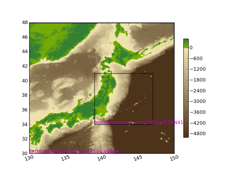
This should reads in two topo files (at resolution 4 minutes and over a smaller region at 1 minute) and plots the topo together. Here is the code:

"""
Sample code to read in two topo files at different resolutions
and plot them together.

Covers the region about the 2011 Tohoku epicenter.
"""

from geotools2 import topoplots
from pylab import savefig

tpd = topoplots.TopoPlotData('testdata/etopo4min130E150E3N48N.asc', topotype=3)
tpd.read()
tpd.cmin = -5000
tpd.cmax = 500
tpd.clf = True
tpd.addcolorbar = True
tpd.plot()

# add another plot from a different file:
tpd.fname = 'testdata/etopo1min139E147E34N41N.asc'
tpd.read()
tpd.clf = False
tpd.addcolorbar = False
tpd.plot()

figfile = "TohokuTopo.png"
savefig(figfile)
print "Created ",figfile

It should create a figure that looks like this:

If you want to be able to zoom in on the figure, it is better to run this code in Ipython, a nice interactive shell for Python:

$ ipython --pylab
In[1]: run test_topoplots_tohoku.py

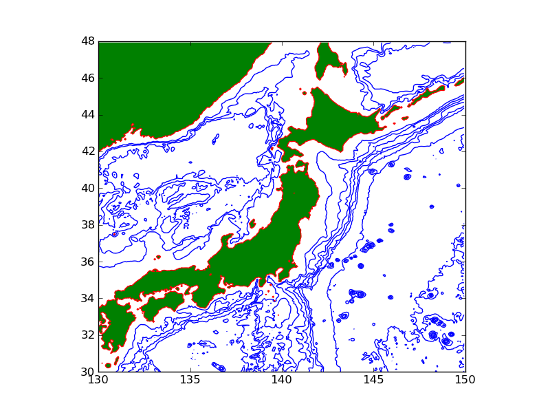
If you want to manipulate the topo data, e.g. to plot something different, you might want to read it in using topotools.topofile2griddata, e.g. as done in this example (found in test_topotools_tohoku.py):

from geotools2 import topotools
from pylab import *

fname = 'testdata/etopo4min130E150E3N48N.asc'

X,Y,Z = topotools.topofile2griddata(fname, topotype=2)

figure(1)
clf()

# plot topography green:
clines = [0,10000]
contourf(X,Y,Z,clines,colors='g')

# plot bathymetry with blue contours:
clines = linspace(-1000,-6000,6)
contour(X,Y,Z,clines,colors='b',linestyles='solid')

# plot coastline red:
clines = [0]   
contour(X,Y,Z,clines,colors='r')

Run this code in IPython and it should produce a plot like this:

Here’s a code that plots contour lines from two different topo file to make it easier to see if the bathymetry matches up well at the edge of the finer grid (found in test_compare_contours.py):

"""
Example comparing contours of bathymetry from two files to 
make sure they match up.
"""

from geotools2 import topotools
from pylab import *

figure(1)
clf()

# first bathymetry file:
fname = 'testdata/etopo4min130E150E3N48N.asc'
X1,Y1,Z1 = topotools.topofile2griddata(fname, topotype=2)

# plot bathymetry with blue contours:
clines = linspace(0,-6000,7)
contour(X1,Y1,Z1,clines,colors='b',linestyles='solid')


# second bathymetry file:
fname = 'testdata/etopo1min139E147E34N41N.asc'
X2,Y2,Z2 = topotools.topofile2griddata(fname, topotype=2)

# plot bathymetry with blue contours:
contour(X2,Y2,Z2,clines,colors='r',linestyles='solid')

Plot in IPython and zoom in to see how well it matches up. Of course you might need to plot different contour levels if you want to see how things look near the coast, for example.