NTHMP Mapping and Modeling Benchmarking Workshop: Tsunami Currents

For GeoClaw code, see the GitHub repository

Results for other problems

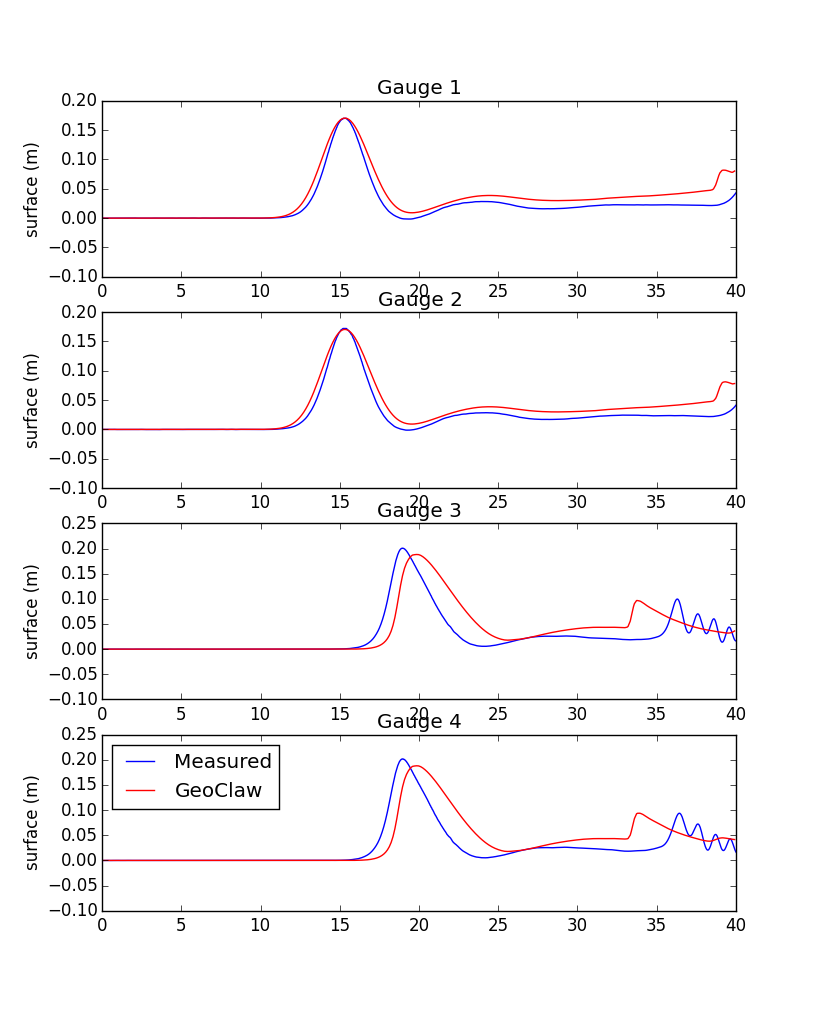
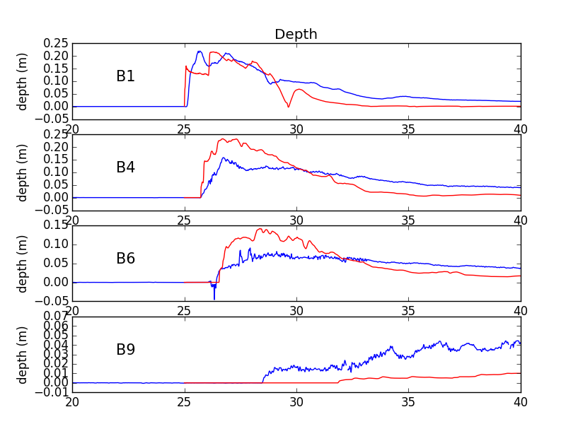
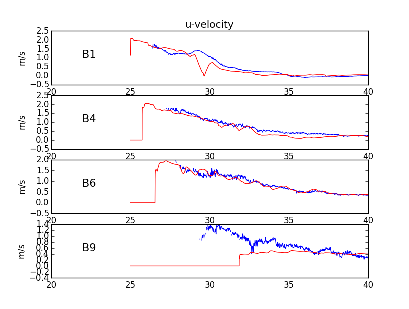
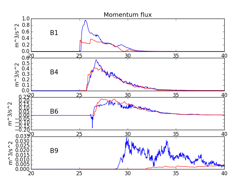
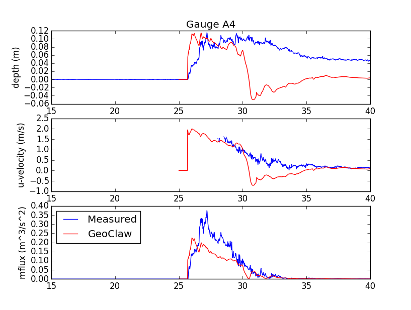
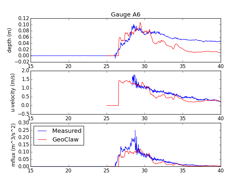
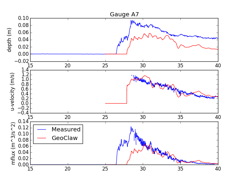
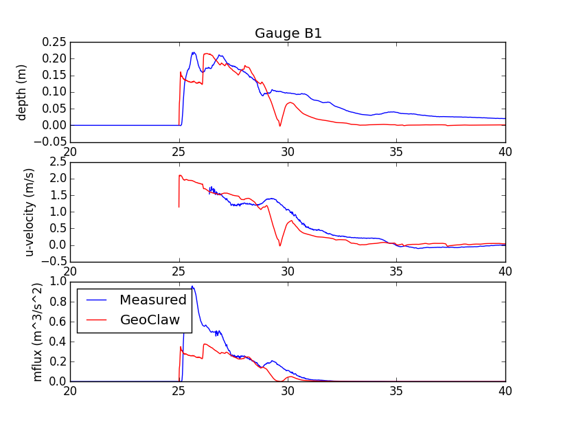
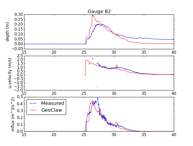
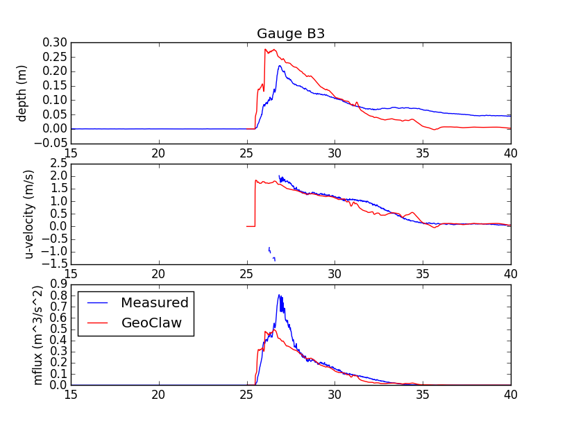
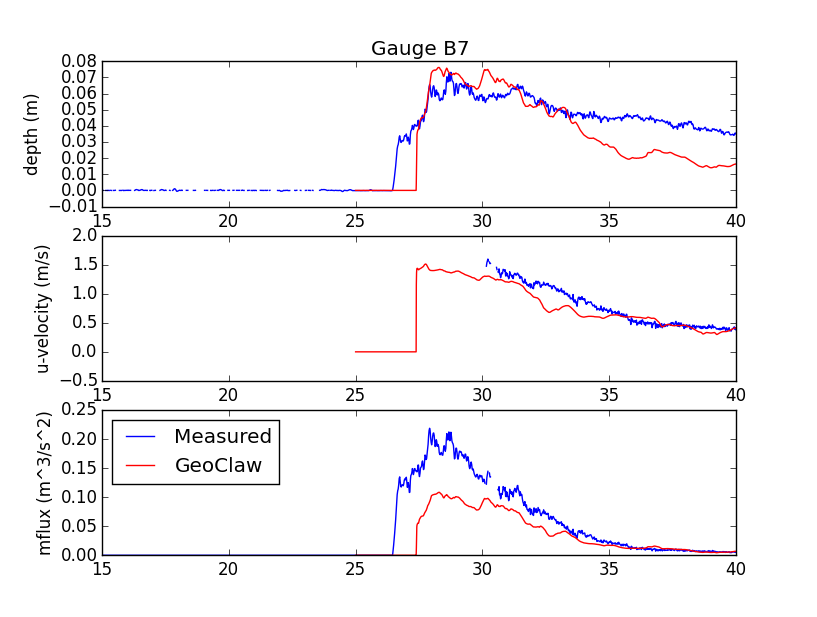
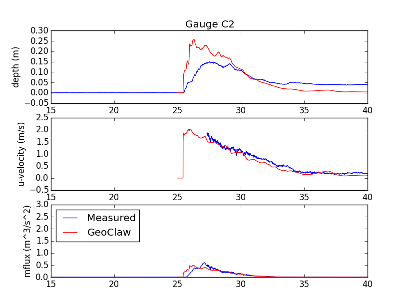
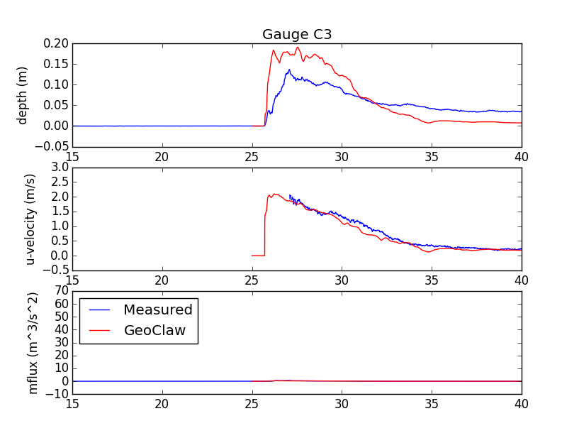
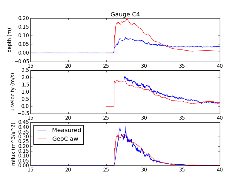
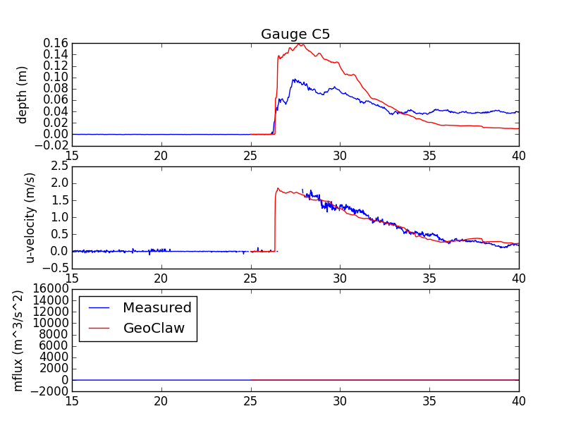
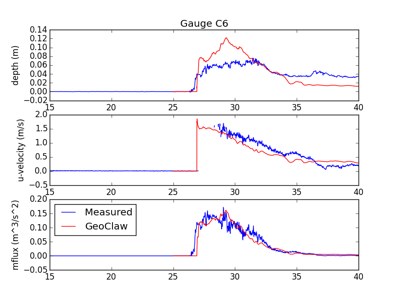
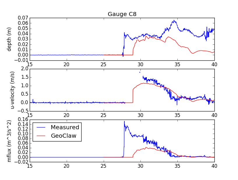
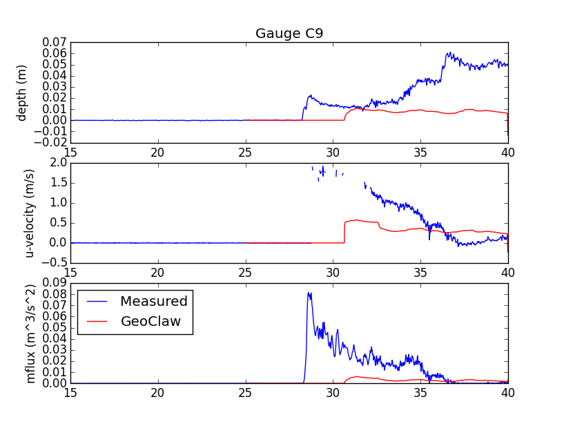
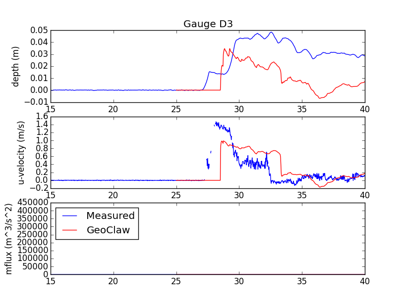
GeoClaw results for Benchmark problem 4

• Problem description

• Full domain animation
• Zoom on Seaside model region
• Wave gauges 1-4

• Depth at B1,4,6,9
• Velocity at B1,4,6,9
• Momentum flux at B1,4,6,9

• Other gauges:
  A1 ... A2 ... A3 ... A4 ... A5 ... A6 ... A7 ... A8 ... A9
  B1 ... B2 ... B3 ... B4 ... B5 ... B6 ... B7 ... B8 ... B9
  C1 ... C2 ... C3 ... C4 ... C5 ... C6 ... C7 ... C8 ... C9
  D1 ... D2 ... D3 ... D4

Notes:

• The data provided for the wavemaker speed \(s(t)\) can be fit quite well with a Gaussian of the form \(s(t) = A \exp(\beta(t - t_0)^2)\) with \(\beta = 0.25, t_0 = 14.75\) and amplitude \(A = 0.51\) [Figure]. However, the amplitude at the Wave Gauge at \(x=5\) matched better in our computation by setting \(A = 0.6.\).

• Adaptive mesh refinement was used. The coarsest grid had a resolution of approximately 0.5 meter cells (\(54 \times 88\) grid cells on the full domain). The finest grid, which only covered the Seaside model region, was refined by a total factor of 40 relative to the coarsest grid (1.25 cm cell size).

• Manning \(n= 0.025\) was used for these results. Still need to test other values.

Work done after the workshop:

Since the workshop we have worked with Mike Motley and his student Xinsheng Qin in the UW Department of Civil and Environmental Energy, to compare our 2D GeoClaw simulations with 3D simulations they have performed using the OpenFOAM software. Results of their work and comparisons of 2D and 3D results are presented in the papers:

• Three-Dimensional Modeling of Tsunami Forces on 2 Coastal Communities, by X. Qin, M. R. Motley, and N. Marafi,

• A comparison of a two-dimensional depth averaged flow model and a three-dimensional RANS model for predicting tsunami inundation, by Xinsheng Qin, Michael R. Motley, Randall J. LeVeque, Frank I. Gonzalez, and Kaspar Mueller.

Two sample animations of a 3D simulation.

Of potential interest to other groups comparing against the experimental data provided for this problem: In the experiment, the peak velocity of the bore front was estimated by analyzing the video data instead of measured by velocimeter, due to air entrained in the bore front. The speed of the bore front is not the same as the peak fluid velocity, which occurs behind the front, and sampling the velocity from the numerical results gives higher peak velocities than the published experimental results. However, Qin, Motley, and Marafi determined that if the video data from the numerical simulation is used to compute the peak velocity in a manner that mimics the experimental procedure, the predicted peak velocity nearly matches the experiment. This is discussed further in their first paper listed above.