Pyclaw Tutorial

Flow of a Pyclaw Simulation

The basic idea of a pyclaw simulation is to construct a Solution object, hand it to a Solver object with the request new time and the solver will take whatever steps are necessary to evolve the solution to the requested time.

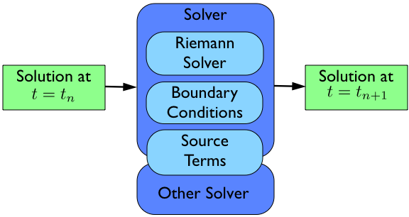
The bulk of the work in order to run a simulation then is the creation and setup of the appropriate Solution objects and the Solver needed to evolve the solution to the requested time.

Note

Here we will assume that you have run import numpy as np before we do any of the tutorial commands.

Creation of a Pyclaw Solution

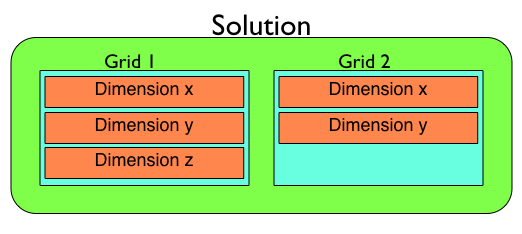
A Pyclaw Solution is a container for a collection of Grid objects in order to support adaptive mesh refinement and multi-block simulations. The Solution object keeps track of a list of Grid objects then and controls the overall input and output of the entire collection of Grid objects. Inside of a Grid object, a set of Dimension objects define the extents and basic grids of the Grid.

The process needed to create a Solution object then follows from the bottom up.

>>> from pyclaw.solution import Solution, Grid, Dimension

>>> x = Dimension('x', -1.0, 1.0, 200)
>>> y = Dimension('y', 0.0, 1.0, 100)
>>> x.mthbc_lower = 2

This code creates two dimensions, a dimension x on the interval [-1.0, 1.0] with 200 grid points and a dimension y on the interval [0.0, 1.0] with 100 grid points. We then set the boundary conditions in the x direction to be periodic (note that if you set periodic boundary conditions, the corresponding lower or upper boundary condition method will be set as well).

Note

Many of the attributes of a Dimension object are set automatically so make sure that the values you want are set by default. Please refer to the Dimension classes definition for what the default values are.

Next we have to create a Grid object that will contain our Dimension objects.

>>> grid = Grid([x,y])
>>> grid.meqn = 2

Here we create a grid with the dimensions we created earlier to make a single 2D Grid object and set the number of equations it will represent to 2. As before, many of the attributes of the Grid object are set automatically.

We now need to set the initial condition q and possibly aux to the correct values. There are multiple convenience functions to help in this, here we will use the method zeros_q() to set all the values of q to zero.

>> sigma = 0.2
>> omega = np.pi
>> grid.zeros_q()
>> q[:,0] = np.cos(omega * grid.x.center)
>> q[:,1] = np.exp(-grid.x.center**2 / sigma**2)

We now have initialized the first entry of q to a cosine function evaluated at the cell centers and the second entry of q to a gaussian, again evaluated at the grid cell centers.

Many Riemann solvers also require information about the problem we are going to run which happen to be grid properties such as the impedence Z and speed of sound c for linear acoustics. We can set these values in the aux_global dictionary in one of two ways. The first way is to set them directly as in:

>>> grid.aux_global['c'] = 1.0
>>> grid.aux_global[`Z`] = 0.25

We can also read in the value from a file similar to how it was done in the previous version of Clawpack. The Grid class provides a convenience routine to do this called set_aux_global() which expects a path to an appropriately formatted data file. The method set_aux_global() will then open the file, parse its contents, and use the names of the data as dictionary keys.

>> grid.set_aux_global('./setprob.data')

Last we have to put our Grid object into a Solution object to complete the process. In this case, since we are not using adaptive mesh refinement or a multi-block algorithm, we do not have multiple grids.

>>> sol = Solution(grid)

We now have a solution ready to be evolved in a Solver object.

Creation of a Pyclaw Solver

A Pyclaw Solver can represent many different types of solvers so here we will concentrate on a 1D, classic Clawpack type of solver. This solver is located in the clawpack module.

First we import the particular solver we want and create it with the default configuration.

>>> from pyclaw.evolve.clawpack import ClawSolver1D
>>> solver = ClawSolver1D()

Next we need to tell the solver which Riemann solver to use from the Riemann solver package . We can always check what Riemann solvers are available to use via the list_riemann_solvers() method. Once we have picked one out, we let the solver pick it out for us via:

>>> solver.set_riemann_solver('acoustics')

In this case we have decided to use the linear acoustics Riemann solver. You can also set your own solver by importing the module that contains it and setting it directly to the rp attribute to the particular function.

>>> import my_rp_module
>>> solver.rp = my_rp_module.my_acoustics_rp

Last we finish up by specifying the specific values for our solver to use.

>>> solver.mthlim = [3,3]
>>> solver.dt = 0.01
>>> solver.cfl_desired = 0.9

In this case, because we are using a Riemann solver that passes back two waves, we must choose two limiters.

If we wanted to control the simulation we could at this point by issuing the following commands:

>>> solver.evolve_to_time(sol,1.0)

This would evolve our solution sol to t = 1.0 but we are then responsible for all output and other setup considerations.

Creating and Running a Simulation with Controller

The Controller coordinates the output and setup of a run with the same parameters as the classic Clawpack. In order to have it control a run, we need only to create the controller, assign it a solver and initial condition, and call the run() method.

>>> from pyclaw.controller import Controller

>>> claw = Controller()
>>> claw.solver = solver
>>> claw.solutions['n'] = sol

Here we have imported and created the Controller class, assigned the Solver and Solution.

These next commands setup the type of output the controller will output. The parameters are similar to the ones found in the classic clawpack claw.data format.

>> claw.outstyle = 1
>> claw.nout = 10
>> claw.tfinal = 1.0

When we are ready to run the simulation, we can call the run() method. It will then run the simulation and output the appropriate time points. If the keep_copy is set to True the controller will keep a copy of each solution output in the frames array. For instance, you can then immediately plot the solutions output into the frames array.

Moving On

This is only a jumping off point for all that can be setup using the pyclaw library. Please refer to the rest of the documentation for more examples and options.