2-dimensional KPP equation

A non-convex flux scalar model

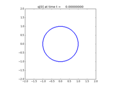
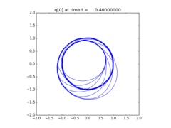
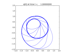
Solve the KPP equation:

\[q_t + (\sin(q))_x + (\cos(q))_y & = 0\]

first proposed by Kurganov, Petrova, and Popov. It is challenging for schemes with low numerical viscosity to capture the solution accurately.

Output:

Source:

#!/usr/bin/env python
# encoding: utf-8
r"""
A non-convex flux scalar model
==============================

Solve the KPP equation:

.. math:: 
    q_t + (\sin(q))_x + (\cos(q))_y & = 0

first proposed by Kurganov, Petrova, and Popov.  It is challenging for schemes
with low numerical viscosity to capture the solution accurately.
"""
from __future__ import absolute_import
import numpy as np
from clawpack import riemann

def setup(use_petsc=False,outdir='./_output',solver_type='classic'):

    if use_petsc:
        import clawpack.petclaw as pyclaw
    else:
        from clawpack import pyclaw

    if solver_type=='sharpclaw':
        solver = pyclaw.SharpClawSolver2D(riemann.kpp_2D)
    else:
        solver = pyclaw.ClawSolver2D(riemann.kpp_2D)
        solver.dimensional_split = 1
        solver.cfl_max = 1.0
        solver.cfl_desired = 0.9
        solver.limiters = pyclaw.limiters.tvd.minmod

    solver.bc_lower[0]=pyclaw.BC.extrap
    solver.bc_upper[0]=pyclaw.BC.extrap
    solver.bc_lower[1]=pyclaw.BC.extrap
    solver.bc_upper[1]=pyclaw.BC.extrap

    # Initialize domain
    mx=200; my=200
    x = pyclaw.Dimension(-2.0,2.0,mx,name='x')
    y = pyclaw.Dimension(-2.0,2.0,my,name='y')
    domain = pyclaw.Domain([x,y])
    state = pyclaw.State(domain,solver.num_eqn)

    # Initial data
    X, Y = state.grid.p_centers
    r = np.sqrt(X**2 + Y**2)
    state.q[0,:,:] = 0.25*np.pi + 3.25*np.pi*(r<=1.0)

    claw = pyclaw.Controller()
    claw.tfinal = 1.0
    claw.solution = pyclaw.Solution(state,domain)
    claw.solver = solver
    claw.setplot = setplot
    claw.keep_copy = True

    return claw

#--------------------------
def setplot(plotdata):
#--------------------------
    """ 
    Specify what is to be plotted at each frame.
    Input:  plotdata, an instance of visclaw.data.ClawPlotData.
    Output: a modified version of plotdata.
    """ 
    from clawpack.visclaw import colormaps

    plotdata.clearfigures()  # clear any old figures,axes,items data

    # Figure for pcolor plot
    plotfigure = plotdata.new_plotfigure(name='q[0]', figno=0)

    # Set up for axes in this figure:
    plotaxes = plotfigure.new_plotaxes()
    plotaxes.title = 'q[0]'
    plotaxes.afteraxes = "plt.axis('scaled')"

    # Set up for item on these axes:
    plotitem = plotaxes.new_plotitem(plot_type='2d_pcolor')
    plotitem.plot_var = 0
    plotitem.pcolor_cmap = colormaps.yellow_red_blue
    plotitem.pcolor_cmin = 0.0
    plotitem.pcolor_cmax = 3.5*3.14
    plotitem.add_colorbar = True
    
    # Figure for contour plot
    plotfigure = plotdata.new_plotfigure(name='contour', figno=1)

    # Set up for axes in this figure:
    plotaxes = plotfigure.new_plotaxes()
    plotaxes.title = 'q[0]'
    plotaxes.afteraxes = "plt.axis('scaled')"

    # Set up for item on these axes:
    plotitem = plotaxes.new_plotitem(plot_type='2d_contour')
    plotitem.plot_var = 0
    plotitem.contour_nlevels = 20
    plotitem.contour_min = 0.01
    plotitem.contour_max = 3.5*3.15
    plotitem.amr_contour_colors = ['b','k','r']
    
    return plotdata


if __name__=="__main__":
    from clawpack.pyclaw.util import run_app_from_main
    output = run_app_from_main(setup,setplot)