Since the alleles are at Hardy-Weinberg frequencies, the frequency of the recessive phenotype = 0.16 = q² (where q = frequency of allele t). Therefore:

q = frequency of t = 0.4

frequency of T = 1 - 0.4 = 0.6

The arithmetic solution to this problem is shown left panel), along with a more general algebraic solution (right panel).

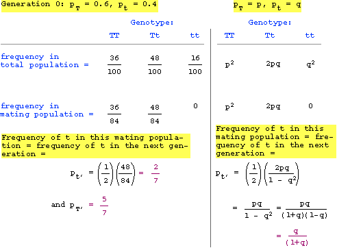
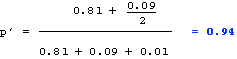
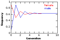
Thus, one generation of restricted mating gives a frequency of T = 5/7 and t = 2/7.

T_n = T₀e^-µn

where T₀ = initial frequency of T = 0.8

e = base of natural log

µ = mutation rate

n = # of generations = 10000

Therefore, after 10000 generations,

frequency of T = 0.8e^-0.02

= 0.784

and the frequency of t = 1 - 0.784 = 0.216

Plugging in the mutation rate, we get N is at least 500,000.

Let the frequency of D = p, and the frequency of d = q, forward mutation rate = u, and back mutation rate = v

Then the change in p would include loss from forward mutation and gain from back mutation; likewise, change in q would include gain from forward mutation and loss from back mutation:

Change in p = vq - up

Change in q = up - vq

At equilibrium, change in p is exactly matched by change in q, so the change in p = 0 (as is the change in q)--

vq - up = 0;

vq = up

Since q = 1 - p, we can substitute and solve for p--

v(1 - p) = up

v - vp = up

up + vp = v

p = v/(u + v)

Therefore, at equilibrium, p = 0.00001/0.00005 = 0.2

q = 1-0.2 = 0.8

Use the frequencies of the various genotype classes--

0.8² x 0.8² = 0.41

2(0.8)(0.2) x 0.2² = 0.0128

2(0.8)(0.2) x 2(0.8)(0.2) = 0.1024

Frequency of baldness allele = q = 0.3

Frequency of wildtype allele = p = 1-0.3 = 0.7

bb = q² = 0.32 = 0.09

Bb = 2pq = 2 x 0.3 x 0.7 = 0.42

BB = p² = 0.7² = 0.49 (where b = baldness allele, B = normal)

Males

Bald = Bb and bb = 2pq + q² = 0.42 + 0.09 = 0.51

Non-bald = BB = p² = 0.49

Females

Bald = bb = q² = 0.09

Not-bald = BB and Bb = p² + 2pq = 0.49 + 0.42 = 0.91

Number of B alleles after immigration = (0.7 x 9000) + (0.1 x 1000) = (6300 + 100) = 6400.

(Actually, since there are 2 alleles per individual, we'd have to double these values -- but the factor of 2 will cancel out in the next step, so we can just ignore that here.)

New value of p = frequency of B in the expanded population = 6400/10000 = 0.64

New value of q = 1-0.64 = 0.36.

Frequency of heterozygotes in the next generation = 2pq = 2 x 0.64 x 0.36 =0.4608

The easy way is to realize that no matter what the father’s genotype, the probability of a heterozygous child is 1/2; therefore, the probability that the child will be a heterozygous carrier is 1/2. If the normal allele is D and the recessive disease allele is d, the mother is Dd and the father could be DD or Dd or dd –

If the father is...	Expected progeny genotypes are...	Probability of Dd child is...
DD	1 DD : 1 Dd	1/2
Dd	1 DD : 2 Dd : 1 dd	1/2
dd	1 Dd : 1 dd	1/2

Thus, regardless of the father’s genotype, the child has a 1/2 chance of being Dd.

Frequency of PKU allele = q = 0.2

For chi-square = 15.625 and df = 1, the P value = 0.0000772265 (this value was obtained from an on-line chi-square calculator). Since this value is well below the usual cut-off value of P= 0.05, we can reject the null hypothesis -- i.e., there is strong statistical evidence that the population does not fit the standard Hardy-Weinberg model.

This is an instance where there appear to be 3 categories -- but all we really need to know is one value (either p or q) and therefore, df = 1 and not 2.

P_tt = q² = 1% = 0.01.

p_t = q = square-root of 0.01 = 0.1

p_T = p = (1 - 0.1) = 0.9

Therefore, P_TT = p² = (0.9 x 0.9) = 0.81

and P_Tt = 2pq = (2 x 0.9 x 0.1) = 0.18

Therefore, the frequency of allele T in the next generation is:

q' = 1 - p' = (1 - 0.94) = 0.06.

p_(Si) = a

p_(Sy) = b

p_(Sg) = c

The distribution of genotypes then is:

(a+b+c)² = a² + 2ab + 2ac + b² + 2bc + c² = 1

               icky          yucky  gross

(Remember that Icky is dominant over everything else, so any animal with allele Si will show the Icky phenotype; etc.)

The frequencies of icky and yucky slugs are compound terms and cannot be calculated directly. However, the frequency of gross slugs = 0.2; c² = 0.2, therefore c = 0.45

But b² + 2bc = 0.3 (= phenotype frequency of yucky slugs)

Substituting for the value of c in this equation, we get

b² + 0.9b - 0.3 = 0

Solving for b, we get b = 0.26.

a = 1 - (b + c) = 0.29.

p_(Si) = 0.29

p_(Sy) = 0.26

p_(Sg) = 0.45

The trend will be as follows: in every generation, the males will show the same allele frequency that the females showed in the previous generation; and the allele frequency in females will be the average of the frequencies in the male and female in the previous generation.

Thus, in generation 0, p_(0f) = 0.9 and p_(0m) = 0.1;

In generation 1, p_(1f) will be 0.5, and p_(1m) will be 0.9

-- note that the D allele frequency in females (0.5) is the mean of 0.9 and 0.1, which were the D allele frequency values in the previous generation, while males show the allele frequency that females showed in the previous generation (0.9)

p_(2f) will be 0.7 and p_(2m) will be 0.5

p_(3f) will be 0.6 and p_(3m) will be 0.7

p_(4f) will be 0.65 and p_(4m) will be 0.6, etc.

These allele frequencies were calculated for each generation the usual way--it is demonstrated for the first generation here:

gametes	0.1D	0.9d	Y
0.9D	0.09DD	0.81Dd	0.9DY
0.1d	0.01Dd	0.09dd	0.1dY
	female progeny		male progeny

p_(1f) = 0.09 + (0.82/2) = 0.5

etc.

Eventually, the frequency of allele D will be the same in males as in females, stabilizing at p = ~0.63 as shown in the graph: