
Until 1966, researchers had only a limited set of tools to look at genetic variation at the gene level.
In 1950, Oliver Smithies invented Gel electrophoresis. A sample of blood or other tissue such as liver or muscle extract is put on a gel made of starch or acrylamide [or some other polymers]. The gel is then put in an electrical field and the proteins migrate according to their charge. The running condition should not denature the protein, so that after a few hours one can stain the gel with unspecific protein stains or add specific substrates for an enzyme, the product then is stained and bands of different mobility are seen.
The bands show how far the proteins have migrated through the gel. The migration distance is a function of the charge of the protein and its conformation. The method can detect single amino acid substitution, but will not detect substitutions that do not change the charge and conformation, of course.
The enzymes produce specific banding patterns dependent on if they are monomers (enzyme is a single molecule), dimers (enzyme consists out of two subunits), tetramers (4 subunits).

The bands are scored and associated with an allele, e.g. alcoholdehydrogenase ADH in Drosophila has a FAST and SLOW allele.
In the early 1960 several studies were showing by electrophoresis that there is variation at some loci. In 1966 Lewontin and Hubby and independently Harris studied electrophoretic variation in populations, Drosophila pseudoobscura, and humans at several loci. And both groups found lots of variation.
Sequencing of the ADH locus (with its F and S alleles; Kreitman 1984) revealed that there were 11 variants with a total of 43 nucleotide substitutions, of which only one in exon 4 accounts for change in the protein sequence and for the F and S polymorphism. Enzyme Electrophoresis reveals only a fraction of the total underlying variability [a picture of this can be seen in Li and Hartl (1991) Fundamental of Molecular Evolution]
the observed Heterozygosity can be calculated as the sum of all heterozygote individuals divided by the total sample. Or, by calculating first the homozygosity (the fraction of the homozygotes) F, and then H = 1 - F. Expected Heterozygosity is calculated by assuming that the population is in Hardy-Weinberg proportions: calculate the allele frequencies and use these to calculate the expected homozygote genotype frequencies. The expected homozygosity is the sum of all homozygote genotype frequencies, H = 1-F.
For multilocus Heterozygosity we simply average the Heterozygosities at each locus.
The polymorphism P is simply the fraction of the loci in which the commonest allele is rarer than 0.95, all rarer alleles add up to more than 0.05. This is quite arbitrary, often a cut-off at 0.99 is also used.
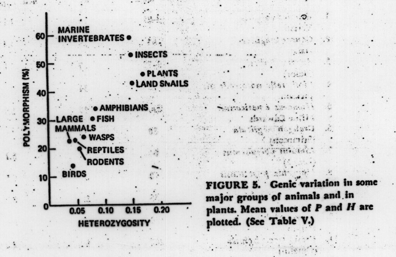
Typical values for heterozygosities in invertebrates are around 15%, about 7% for vertebrates. The variation of these overall averages is very high, for example in amphibian we can find H > 15% based on enzyme electrophoresis.
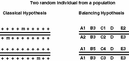
The results of the first enzyme electrophoretic surveys invalidated Muller's hypothesis. Lewontin made an argument that Dobzhansky's hypothesis may be not correct too: If we believe that there is strong balancing selection than we have fitnesses for the different genotypes at a single locus AA: 1-s1, Aa: 1, aa: 1-s2, this results in a population fitness smaller than 1 (w < 1). If we take an organism with 10000 genes and perhaps about 30% are polymorphic and assume that the fitnesses are multiplicative than we can calculate the overall fitness w* = w1 * w2 * ..... *wn. Since the w for each locus are smaller than one the overall fitness w* <<<< 1. This would suggest that a randomly chosen individual may be less fit by magnitudes, which is not what one can see in experiments.