Most of the following is work derived by Motoo Kimura the architect of the neutral theory. Most change in a population is due to mutations that are selectively neutral.
Kimura derived the fixation probability P for an allele under random genetic drift and genic selection, with fitnesses for the genotypes w(AA)=1, w(Aa)=1+s, w(aa)=1+2s, where s is the selection coefficient and it can be positiv [advantageous] or negative [deleterious]. q is the initial allele frequency of a
| 1 - exp(-4Nsq) | |
| P(a)= | ----------------- |
| 1 - exp(-4Ns) |
This rather complicated formula, simplifies considerably, if we are willing to make some simplifying assumptions:
|
s approaches 0.0 [exp(-x) is approx. 1-x when x is small] |
|
The fixation probability under a neutral mutation regime is exactly the initial allele frequency.
In a population of N diploid individuals, and a (single) new mutation arises, this mutation has an allele frequency of
| 1 |
| ----- |
| 2N |
If we replace q with 1/2N then we can investigate what happens under selection
|
s > 0.0, and N is large [If N is large exp(-4Ns) goes to 0.0] |
|
If we plug in numbers, we can see that that if a new beneficial mutant has a selection coefficient of 1% (under genic selection this means that the heterozygote Aa is 1% more fit than AA and aa is 2% more fit than AA) there will be only a chance of 2% that this allele will fix [the exact formula delivers for N=100 a value of 2.02%], and in 98 of 100 cases this beneficial allele gets lost.
If we inspect the complicated first formula again then we can also calculate what the fixation probability for a deleterious allele would be [the simplification in formula 3 assume that the mutation is beneficial]. We plug in numbers into the first formula using q=1/2N, s = -0.01, N is 100, and get P(a[deleterious]) = 0.0004. In large populations the fixation probability for a deleterious allele is very small [try yourself].
The fixation of a benefical mutation is independent by the population size (under the assumption that the population is not too small). The chance of fixation of a deleterious allele is small in large populations, but rather high in small populations.
We inspect (conditional) time to fixation of an allele of which we know (by some oracle) that it will eventually fix. Kimura and Ohta found that the average time t of fixation
where ln() is the natural logarithm.
Example: N=106, s=0.01, then t(neutral)=4 * 106 generations, and t(selected) = 2901 generations.
If we know that an allele will fix than under a neutral regime it will take an awful long time to fix, whereas under slight selection it zooms to fixation.
As a result of the above we can expect that neutral mutations stay a rather long time in the population and eventually one or the other gets fixed or lost due to genetic drift. There is a constant turnover of alleles and none of the individual allele frequeuncies stayes fixed over time.
There is a (roughly) constant overall level of heterozygosity, that depends on the population size.
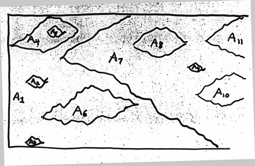
| gene copies along y axis |
|
| Time |
In a random-mating population of size N with neutral mutation a fraction F of the pairs of copies will be homozygous. Suppose all mutations create completely new alleles, and the rate of these neutral mutations is u. Then a pair has by chance the same parent in the last generation with probability 1/(2N) and has NOT the same parent with 1-1/(2N). To be identical, both copies must not be new mutations and the probabiity of this is (1-u)(1-u). We can set up a recurrence equation
At equilibrium (F'=F) we can solve the equation and get
| (1-u)2(1/(2N)) | |
| F = | ------------------------ |
| 1 - (1-u)2(1- 1/(2N)) |
| 1 | |
| F = | --------- |
| 1+ 4Nu |
the heterozygosity H is 1- F :
| 4Nu | |
| H = | --------- |
| 1+ 4Nu |
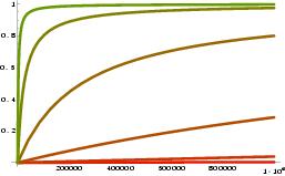
Example graph: y-axis is heterozygosity, x-axis population size, each line is a different mutation rate: from the bottom to the top: u=10-8, 10-7, 10-6, 10-5, 10-4.
Not all individual in a population reproduce. We were using N as the population size, but need to refine this concept, because in our earlier examples we assumed that all individuals produce gametes and have potential offspring. The census population size is the number of individuals in a population. We are more interested in the numbers of those who contribute to the next generation. We use the effective population size Nefor these. The effective population size depends on the sex ratio and the reproduction mechanism. For example, a strictly selfing species would have a Ne=1, because all offspring are perfect copies of their Ur-mother.
In sexual species with no selfing the relationship between Ne and the sizes for each sex (Nf(emales),Nm(ales)) is
| 4 NfNm | |
| Ne = | --------- |
| Nf + Nm |
Example: Assume we have a species with a sex ratio if 1:1 and a total of 2000 individuals, then we calculate an Ne of 2000, if the sexratio is skewed to 1:100 we get only an Ne of 39.604.
Over history we do not expect that natural populations stay constant, there will be some fluctuations over the generations, due to environmental changes, diseases, famines, good years, ... When the population grows the alleles present will most likely not go extinct that quickly and with time new alleles will increase the expected heterozygosity. With bottlenecks, reduction of the population size many allleles fix or get lost quickly, and the heterozygosity and the effective population size is lowered. Over many generations the overall effective population size depends more on the small effective population sizes, it is the harmonic mean
(Ne = n/(1/N1+1/N2+...+Nn)
where n is the number of generations.