Lecture January 5: Hardy-Weinberg Proportions

Hardy-Weinberg Proportions

HWP are based on following assumptions:

Single random mating population
Infinitely many individuals
No mutation
No selection (no differential fertility, viability)
No immigration or emmigration
Non-overlapping generations

Example Phenotype (codominant)	White	Pink	Red
Example Phenotype (dominant)	White	White	Red
Genotypes	AA	Aa	aa
Observed numbers	N_AA	N_Aa	N_aa
Genotype frequency	N_AA/N	N_Aa/N	N_aa/N	N=N_AA+N_Aa+N_aa
	P	H	Q	P+H+Q=1

Allele	A	a
Allele frequency	p_A [we use often just p]	p_a [we use often just q]	p_A+p_a=1
	P + 0.5 H	Q + 0.5 H
	(2 N_AA + N_Aa) ----------- 2 N	(2 N_aa + N_Aa) ----------- 2 N

If the mentioned assumptions hold then the Hardy-Weinberg proportions are achieved in one generation, and after that the allele frequencies stay the same in all future generations.

Example 1: MN red blood cell locus

The observed numbers and the numbers expected from Hardy-Weinberg proportions for the MN blood group locus in an English sample of 1000 blood donors (from Cleghorn 1960)

Phenotype	Genotype	Observed Number	Expected Number
M	MM	298	ppT=294.3
MN	MN	489	2pq*T=496.3
N	NN	213	qqT=209.3
Total T		1000	1000

Use the "Algebra of the Hardy-Weinberg Equilibrium" to calculate the p and q of the MN blood locus example.

Calculation of allele frequencies for cases with a dominant allele

If we assume that a population IS in Hardy-Weinberg proportions (HWP) then we can calculate the allele frequencies even in cases where one allele is dominant and we cannot distinguish between heterozygotes and the dominant homozygote. We use the fact that the frequency of the recessive allele (say a) has

P_aa = (frequency(a))² = q²
q = frequency(a) = Sqrt(P_aa)

In Example 2 we calculate for the recessive allele + in the life frogs is
P_aa = 834 / (834 + 53) = 0.940248
allele frequency q = p_aa = Sqrt(0.940248) = 0.969664
the dominant allele is p=1-q.

Example 2: Coloration variants in frogs (Rana pipiens)

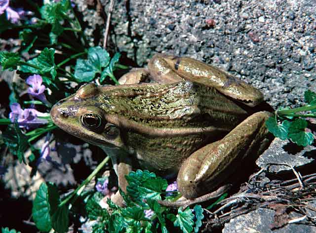Two color morphs (alleles B and +) of the leopard frog (Rana pipiens). The allele B is dominant, heterozygotes (B+) look like BB. The study was done in Minnesota and investigated if there were differences in in HWP between animals found dead compared to animals caught alive.
On the left the common subspecies (R. p. pipiens), on the right R. p. burnsi. Adapted from Hedrick (2000), data is from Merrell and Rodell (1968). Pictures are (c) Jeff LeClere.

	Phenotype	Genotype	Observed Number	Allele Frequency
Living	burnsi	BB, B+	53	0.030
	pipiens	++	834	0.970
Dead	burnsi	BB,B+	39	0.018
	pipiens	++	1050	0.982

Hardy-Weinberg proportions with multiple alleles

Example with 3 alleles
Genotypes	A₁A₁	A₁A₂	A₁A₃	A₂A₂	A₂A₃	A₃A₃
Genotype Frequencies	P₁₁	P₁₂	P₁₃	P₂₂	P₂₃	P₃₃

p(A₁) = frequency(A₁) = P₁₁ + 0.5 P₁₂ + 0.5 P₁₃)

p(A₂) = frequency(A₂) = P₂₂ + 0.5 P₁₂ + 0.5 P₂₃)

p(A₃) = frequency(A₃) = P₃₃ + 0.5 P₁₃ + 0.5 P₂₃)

p(A_i) = frequency(A_i) = P_ii + 0.5 Sum^k_{j,i ≠ j}(P_ij)

Heterozygosity

The number of heterozygotes in a sample can be used as a measure of variability. The OBSERVED heterozygosity H is simply the frequency of the heterozygotes in the sample. If we assume HWP then the EXPECTED heterosygosity is 2pq for two alleles. For multiple alleles it is often easier to subtract the homozygote genotypes from 1, in general

H_exp= 1 - Sum(P_ii)

In Example 2 the dominant allele is masking the heterozygotes, assuming that the population is in HWP, we can calculate the expected heterozygosity H = 2 * 0.969664 * 0.0303361 = 0.0588317 and by multiplying this with the total number (834+53) we estimate the number of heterozygotes as 52 (52.18). Most likely there is only one homozygote burnsi in the living frog sample. This is a common situation, rare alleles most often occur in a heteroyzgote.

Deviation of Hardy-Weinberg porportions

We can test if a sample is in HWP by using a Chi²-Test with the Null hypothesis H₀: Sample is in HWP, and the alternative hypothesis H₁: Sample is NOT in HWP. For date sets with multiple allele one wants to use more sophisticated procedures, such as those by Guo and Thompson (1996). We use the following

 
                      (Observed - Expected)²
Chi² = Sum -------------------------------
                           Expected

The sum is over all genotypic classes. From the calculated Chi² and with knowledge of another number, the degrees of freedom, we can obtain by comparison with a tabulated Chi² the probability that the observed numbers deviates from the expected numbers as much or more by chance. The degree of freedom is the number of classes minus 1 and then minus the number of parameters estimated from the data. For the two allele case we have 3 genotypic classes (P_AA,P_Aa,P_aa) of which one can be calculated by knowing the other two. We have one parameter p_A (we can calculate the other as p_a=1-p_A). This results in 1 degree of freedom (3-1 - 1). If we use a significance level of 5% (we will erroneously accepting the alternative hypothesis in 5% of all tested cases) the tabulated Chi² is 3.84. We will accept the alternative hypothesis when our testvalue is bigger than the tabulated one.
In the two allele case we calculate

	(P_AA - p²)²		(P_Aa - 2pq)²		(P_aa - q²)²
Chi² =	-----------------	+	-----------------	+	-----------------
	p²		2pq		q²

The follwing numbers are from Example 1, remark the use of observed and expeted numbers instead of frequencies.

	(298 - 294.3)²		(489 - 496.3)²		(213 - 209.3)²
Chi² =	-----------------	+	-----------------	+	-----------------	= 0.015
	294.3		496.3		209.3

The calculated testvalue is smaller than the tabulated chi² value and we will reject the alternative hypothesis and believe that the MN Blood locus is in HWP proportions.

Possible explanation for deviation of HWP are violations of the assumptions, for example influences of

Selection
Non-random mating
Gene flow
etc.

In surveys of natural populations we often find that populations are in HWP. When a population is in HWP we cannot say that there is no selection or non-random mating working.