Sample results for Quillayute River flooding

Example from https://github.com/rjleveque/csdms_clinic_2024. The code to run this test is in the quiallayute subdirectory.

Test problem setting up a steady state flow in the Quillayute River that flows into the Pacific Ocean at La Push, WA (in the Quileute Tribal Nation).

This is a region in danger of flooding, where remediation efforts are underway. See for example this story, which includes a good Google Earth image of a potentially flooded region.

%matplotlib inline

from pylab import *

Plot topography DEM

If you are using the CSDMS JupyterHub, select the Clawpack kernel before running this notebook in order to import clawpack modules. (The kernel appears in the top-right corner of the notebook, click on it to get a menu of possible kernels.) This kernel also includes pylab and matplotlib.

Note that the topography file Quillayute_13s.asc will not be found unless you run make topo in a terminal window.

from clawpack.geoclaw import topotools

topo = topotools.Topography('Quillayute_13s.asc', topo_type=3)

fig,ax = subplots(figsize=(10,4))
topo.plot(axes=ax, limits=[-20,20], cb_kwargs={'extend':'both'})
title('Topography DEM (0 = MHW)');

View plots in notebook

After running make .plots, the _plots directory contains plots that can be viewed by opening the html file _plots/_PlotIndex.html.

This notebook can be used if you are on a JupyterHub where you are not able to open that file to view the plots.

Also, on the CSDMS JupyterHub you can obtain the plots and output directories using the following command in a terminal window:

cp -r /data/quillayute/_* ./

This is useful since OpenMP is not available on the JupyterHub computer and so the codes run much more slowly than on a laptop.

#from clawpack.clawutil import nbtools
# The tools we need aren't in clawpack yet, so use the local version:
import sys
sys.path.insert(0, '..')
import nbtools

plotdir = '_plots'

Initial conditions:

The water depth is initialized based on the topography (which is referenced to MHW), so the part of the river where the river bed is below MHW has water in it and the rest is dry.

nbtools.show_frame(frameno=0, figno=1, plotdir=plotdir)

'

Evolution of depth:

Note that AMR patch edges are shown levels 2 and 3 (refinement by 4 at each level).

for frameno in range(1,4):
    print('Frame %i:' % frameno)
    nbtools.show_frame(frameno, figno=0, plotdir=plotdir)

Frame 1:

'

Frame 2:

'

Frame 3:

'

Zoom near La Push

We see that a steady state is approached over the first hour

for frameno in range(2,7,2):
    nbtools.show_frame(frameno, figno=1, plotdir=plotdir)

'

'

'

Gauge plots

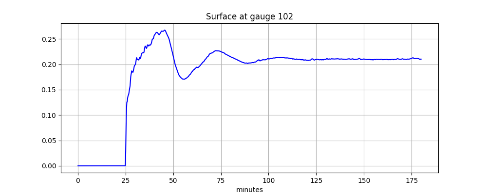
Time series at the two synthetic gauges 101 and 102 shown in the plots above show the evolution of the water surface.

for gaugeno in [101,102]:
    nbtools.show_gauge(gaugeno, width_percent=70, plotdir=plotdir)

'

'

One hour is not long enough to reach steady state flow, 2-3 hours are needed for this problem. Running the code out longer shows this time series at Gauge 102, for example:

Animation over the full domain:

These plots also show the AMR patch boundaries. Note that the river source region is shown by the yellow rectangle near the right edge of the domain.

nbtools.show_movie(figno=0, width_percent=100, height_pixels=600, plotdir=plotdir)

<embed src='_plots/movie_fig0.html' width='100%%' height='600px' />

Add flooding event

Re-running the code via:

make -f Makefile_flood
make data -f Makefile_flood
make output -f Makefile_flood
make plots -f Makefile_flood

adds a major precipitation event east of -124.59 with a duration of 15 minutes starting at 1 hour. Then the plots below should be available in _plots_flood.

plotdir = '_plots_flood'

for frameno in range(4,9,2):
    nbtools.show_frame(frameno, figno=0, plotdir=plotdir)

'

'

'

Animations of the La Push region:

nbtools.show_movie(figno=1, plotdir=plotdir, width_percent=100, height_pixels=600)

<embed src='_plots_flood/movie_fig1.html' width='100%%' height='600px' />

nbtools.show_movie(figno=11, plotdir=plotdir, width_percent=100, height_pixels=600)

<embed src='_plots_flood/movie_fig11.html' width='100%%' height='600px' />

Gauge plots:

for gaugeno in [101,102]:
    nbtools.show_gauge(gaugeno, plotdir=plotdir, width_percent=70)

'

'