Introducing the ATK: Imaging illustrations Extension
ExtensionThe material here was originally included as part of Introducing the Ambisonic Toolkit, and has been lightly edited. This discussion concerns how to intrepret the figures accompanying a number of First Order Ambisonic (FOA) imaging UGens.
Reading imaging illustrations
As artists working with sound, we should expect most users to be very capable expert listeners, and able to audition the results of spatial filtering of an input soundfield. However, it is often very convenient to view a visual representation of the effect of a soundfield transform. The ATK illustrates a number of its included transforms in the form shown below.
The X-Y axis is shown, as viewed from above with the top of the plot corresponding to the front of the soundfield, +X. On the left hand side of the figures, an unchanged soundfield composed of eight planewave is shown. These are indicated as coloured circles, and arrive from cardinal directions:
- Front
- Front-Left
- Left
- Back-Left
- Back
- Back-Right
- Right
- Front-Right
Three useful features are displayed in these plots, providing inportant insight as to how an input soundfield will be modified by a transform:
- incidence1 : illustrated as polar angle
- quality2 : illustrated as radius
- gain3 : illustrated via colour
Individual planewaves are coloured with respect to the gain scale at the far left of the figures. Additionally, Front, Left, Back-Left and Back are annotated with a numerical figure for gain, in dB.
Soundfield quality
The meaning of transformation to soundfield incidence and gain should be clear. Understading the meaning of soundfield quality takes a little more effort. This feature describes how apparently localised an element in some direction will appear.
A planewave has a quality measure of 1.0, and is heard as localised. At the opposite end of the scale, with a quality measure of 0.0, is an omnidirectional soundfield. This is heard to be without direction or "in the head". As you'd expect, intermediate measures are heard as scaled between these two extremes.
You may like to review the ATK Glossary for further descriptions and definitions.
Reading ZoomX
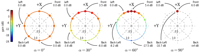
ZoomX imaging
With changing ZoomX's angle, we see the eight cardinal planewaves both move towards the front of the image and change gain. When angle is 90 degrees, the gain of the planewave at Front has been increased by 6dB, while Back has disappeared.4 We also see the soundfield appears to have collapsed to a single planewave, incident at 0 degrees.5
Reading PushX
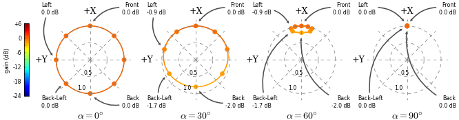
PushX imaging
PushX also distorts the incident angles of the cardinal planewaves. However, here we see two differences with ZoomX. The gains of the individual elements don't vary as considerably. More intriguingly, a number of the encoded planewaves are illustrated as moving off the perimeter of the plot, indicating a change in soundfield quality.
Moving from the edge of the plot towards the centre does not imply the sound moves from the edge of the loudspeakers towards the centre, as one might expect. Instead, what we are seeing is the loss of directivity. Moving towards the centre means a planewave moves toward becoming omnidirectional, or without direction. (This becomes clearer when we look at DirectO.) A reducing radius indicates a reducing soundfield quality.
When PushX's angle is 90 degrees, all encoded planewaves have been pushed to the front of the image. Unlike ZoomX, gain is retained at 0 dB for all elements.6
Reading DirectO
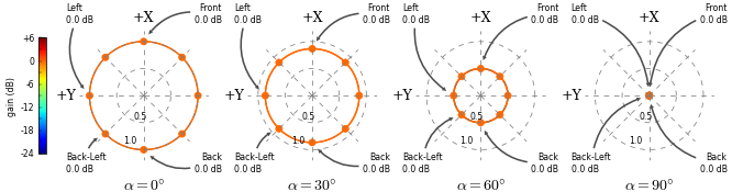
DirectO imaging
DirectO adjusts the directivity of the soundfield across the origin. Here we see the cardinal planewaves collapsing towards the centre of the plot. At this point the soundfield is omnidirectional, or directionless. See further discussion of soundfield quality above.
See FoaZoomX, FoaPushX and FoaDirectO for more details regarding use of these associated UGens.
Illustrated transforms
For your reference, the following UGens include figures illustration imaging transformation:
Do take the time to explore these to get a sense of the wide variety of first order image transformation tools available in the ATK.
link::Guides/Reading-FOA-Imaging::