Rocks might have lots of different magnetic particles in them. They might contain magnetite, an iron oxide that forms in igneous and metamorphic rocks as well as in soils; they might contain titanomagnetite, a common consitituent of oceanic basalt; they might contain maghemite that formed as magnetite was oxidized — rusted — by weathering, or they might contain maghemite that formed in soils; they might contain hematite or goethite, indicating soil formation in dryer or wetter environments… there are even rock-forming minerals like pyroxenes and micas that are magnetic to a certain extent. In addition to forming in different environmental conditions, all of these minerals have particular quirks in their record of Earth’s magnetic field. So we need to be able to tell the kinds of magnetic minerals apart.
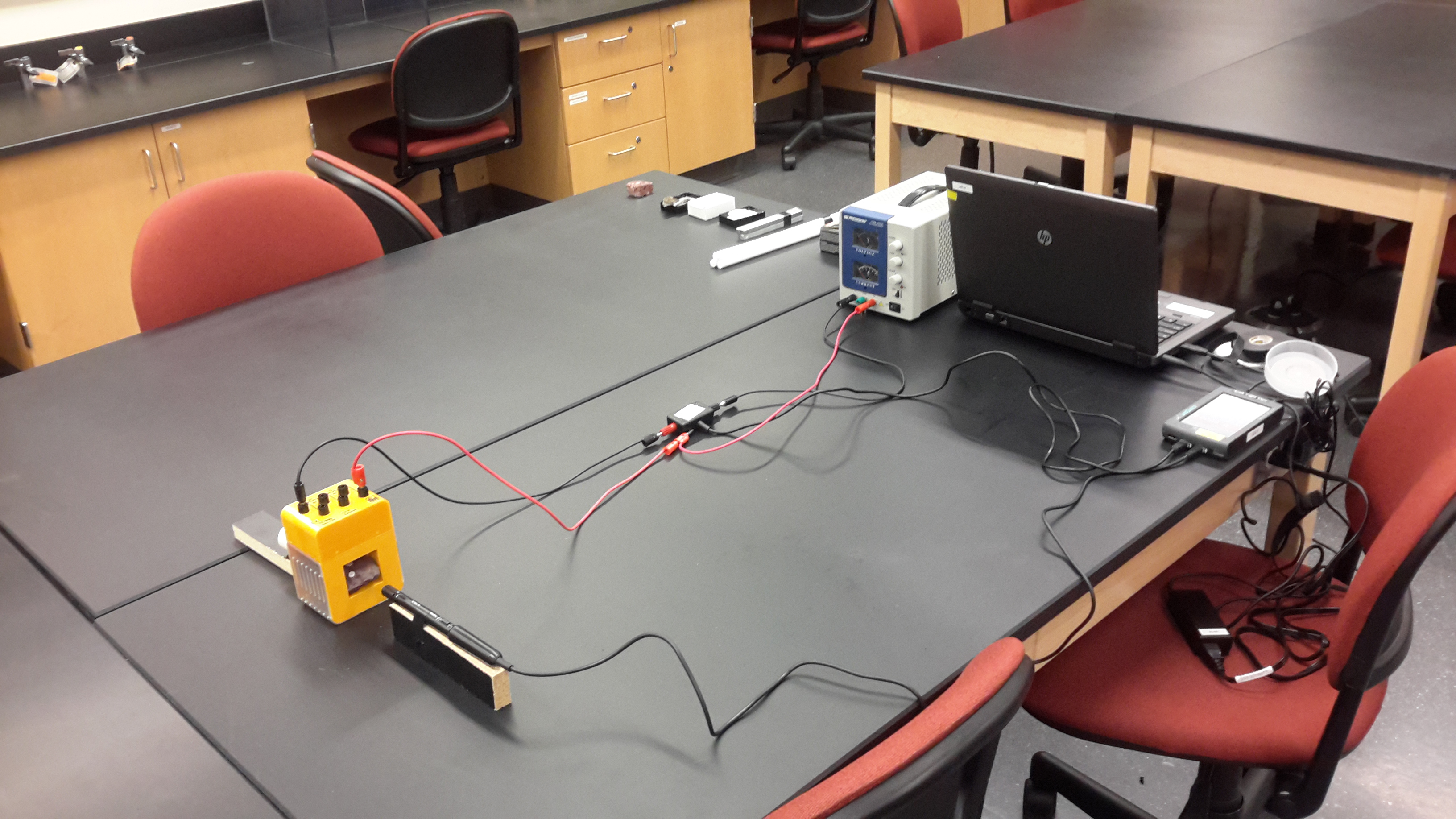
One way we differentiate between magnetic minerals is by their response to weak magnetic fields. So I tried a little experiment. I put a bunch of different materials inside a wire coil. I could send a current through the coil, producing a (weak) magnetic field at the coil’s center. I also set up a magnetometer to measure the magnetic field just outside the coil.
Why might the field inside the coil be different from what I measure with the magnetometer? This is a secret that is not addresed in the physics textbook we use in Physics II: there are two different ways of describing magnetic fields. We call the magnetic field that the magnetometer 


")
There are two ways you can get a little bit of extra field from putting stuff inside the coil. A large number of Earth materials become magnetic when you put them in a magnetic field, but then revert to what most people would call “non-magnetic” when the magnetic field is turned off. For example, if you put an iron-bearing garnet crystal inside an area with zero magnetic field, it wouldn’t attract a compass needle. But as soon as you turn the magnetic field on, the compass needle begins to deflect – ever so slightly – toward the garnet. We call that garnet paramagnetic. Other minerals, like quartz, are diamagnetic: put them in a magnetic field, and the compass needle deflects away from the mineral. For both paramagnetic and diamagnetic materials, the effect on the compass disappears when you shut off the magnetic field you’ve applied. We call this an induced magnetization.
Some materials also have a remanent magnetization – a magnetization that remains after the
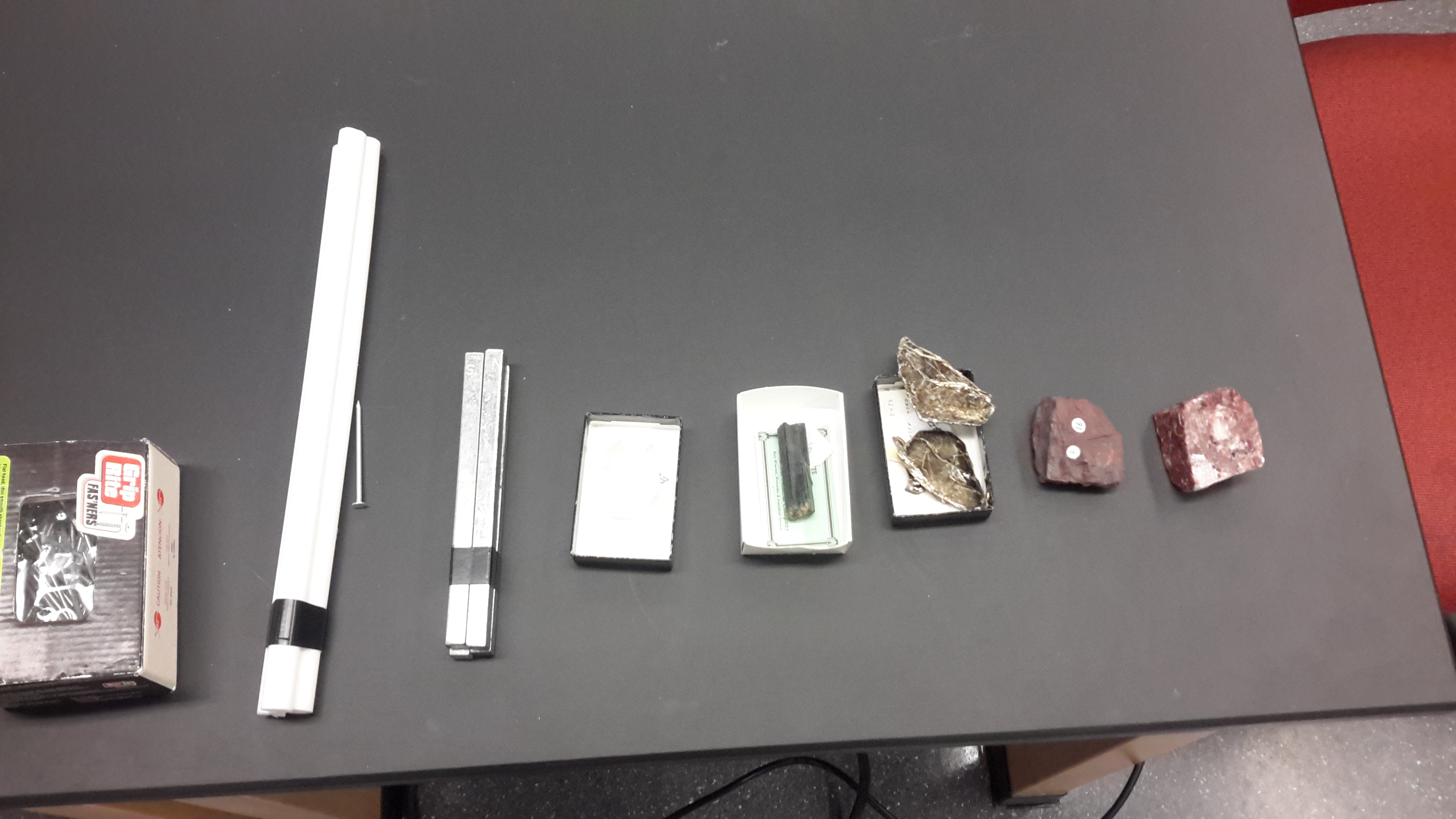
So: I took pieces of a bunch of different materials – steel, teflon, hematite, and various other minerals – and put them in the middle of the coil to see what would happen to the magnetic field as I increased and decreased the current. I tried the mica in two different directions (with the edge pointed toward the magnetometer, and with the flat face 45° from the magnetometer) to see if there was an effect.
Here is a plot illustrating the response of these materials to the magnetic fields produced in the coil:
The first thing you might notice is that all materials, more or less, make a linear trend on this plot. So the total magnetic field is proportional to the applied field. The biggest effect is in the bar magnets: they are ferromagnetic (the line of points does not intersect the origin, meaning that there is some magnetic field that remains when you turn off the
The ratio between applied magnetic field and a material’s (induced) magnetization is called magnetic susceptibility. It is given the symbols k, κ, or χ. If you were to measure magnetic susceptibility carefully, you could identify differences between these minerals – perhaps even between the different orientations of the mica. To do that, you need to have a good idea about what the response of your magnetometer would be if your coil were empty. That’s your model for how your measurement device works. It’s just a linear equation here: 

Here is what you get when you subtract out the empty sample holder’s response:
On these graphs, a positive slope indicates a material that behaves as a paramagnet; a negative slope indicates a diamagnet. Most of these materials behave like a combination of the two – not a particularly steep positive slope (except for the bar magnets) and a variety of negative slopes. The Teflon rods have the steepest negative slope because they contain the most diamagnetic material. Because ferromagnetic materials retain a 
Here is the R code for the graphs:
…and the data file.
]]>]]>I highly recommend that everyone who goes through my lab learn how to explain their project to the public. This is partially because you’ll have to do it when you get to Senior Seminar (TESC 410). Evan more importantly, it’s because we scientists need to be better about engaging the public with our science. If we don’t, we run the risk of becoming the kind of caricature of a scientist you see in the movies: academics with no connection to the real world.
So, to make that connection with the public, we have a blog. Or rather, I do, since I’m the one who usually writes for it. I try to explain what’s exciting about my science in a way that college students taking an intro class (or any interested people at about that level) might understand. The audience I write for isn’t stupid, but they might not be familiar with the jargon we use as scientists and the kinds of graphs we show each other. They might not care about the details of my work, but they do care about what’s new, exciting, or potentially relevant. Why I do things is much more relevant than how I do them. My audience also cares about stories (I think), including stories about how science works for me.
There are no strict rules about writing a blog post. This is an assignment with no strict page limit or style guidelines. Really, it’s the ideas and how you convey them that matters. I’ve seen a lot of good material on how to run a blog in general. I’m collecting it below. Some of it might be helpful if you’re writing a single post. In the broader sense of communicating your science, I’ve found some useful guidelines in Nancy Baron‘s book Escaping the Ivory Tower. Baron directs an influential program called COMPASS that focuses on preparing scientists to better communicate with the public. Her book has a lot of useful information about how to make sure your science is relevant to different audiences (politicians, journalists, filmmakers, etc.).
- Blogging tips for science bloggers, from science bloggers, by Paige Brown Jarreau (@FromTheLabBench on Twitter, where she posts lots of good science communication analysis and advice)
- Example blogs by scientists, in no particular order:
- Becker Lab
- Emily Lakdawalla at the Planetary Society
- Callan Bentley’s Mountain Beltway
- Georneys by Evelyn Mervine
- On Circulation (group blog, I think)
- Simon Wellings’ Metageologist (my current favorite: he has a great introductory post on the Bengal Fan)
One of COMPASS’s signature tools is the Message Box, a scheme for organizing your scientific ideas so you can pitch them to non-scientist readers. Working your ideas into a message box is hard. But it’s good preparation for writing a blog post. Plus it forces you to think about how your science s relevant… which is the whole purpose of doing it! If you want to give the message box a try, there is a template here.
Guidelines:
Aim for about a page of text, with an image. If you don’t have an image, I can help.
You can use informal language, but don’t be sloppy. People will read this.
Have you taken pictures? Drawn comics? Found places on Google Maps? Great! I’m a visual person, and I like having good images on the blog.
Aim to engage people rather than to explain. Stories are good.
Avoid jargon, but don’t dumb it down. Explain it when you have to. I think of my posts as initiating readers into the club of people who understand what I’m talking about.
Look at other blog posts for inspiration.
 ]]>
]]>

[1] Previous relevant posts are under the paleomagnetism tag.
]]>
Note: this is not at all exhaustive or up to date. I’m trying to choose articles that I’d give to students who are taking or about to take a middle-division course in geology (e.g. sedimentology). These are not necessarily the earliest or latest, or the most relevant to the specific things we’re doing out here, but these will get you started. I may introduce a couple of more specific key ideas in future blog posts. Watch this space for more. Email me or comment if you have any suggestions!
First, if you’re just a casual reader who may be interested in working with me on a project when I get back, you might start with Diane Hanano’s blog post on deep drilling.
For a big-picture view of the growth of the Himalaya and some of the questions geologists have about it: Molnar, P. (1997) The rise of the Tibetan Plateau: From Mantle Dynamics to the Indian Monsoon. Astronomy and Geophysics 38:10-15. (Link)
Why we care about the erosion of the Himalaya: Raymo, M.E., and W.F. Ruddiman (1992) Tectonic forcing of late Cenozoic climate. Nature 359: 117-122.
For a summary of the sedimentary processes occurring on the Bengal Fan itself, with lots of maps: Curray, J.R., F.J. Emmel, and D.G. Moore. (2003) The Bengal Fan: morphology, geometry, stratigraphy, history and processes. Marine and Petroleum Geology 19: 1191-1223.
]]>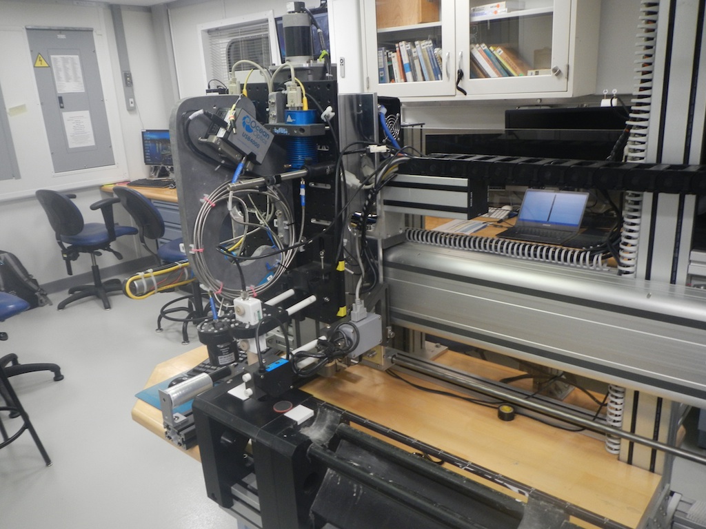
This is an instrument that records the color and magnetic susceptibility of split cores (“section halves”) [2]. It’s actually a robot that slides along a track taking measurements. We call it the Section Half Multi Sensor Logger, or SHMSL (pronounced “schmizzel”). The Germans on board have started calling it the Schnitzel.
The SHMSL isn’t really in our lab, but we use data from it all the time. In fact, there’s a back-and-forth between all of the labs on the ship. Paleontologists use the ages when plankton species appear and disappear from the fossil record to help us narrow down which magnetic reversals we’re measuring. We talk to the sedimentologists about sedimentation rate and what kinds of (magnetic) minerals might be in the sediments. The physical properties scientists help us decipher seismic reflection diagrams – more on those later – and collect most of the magnetic susceptibility data (three of the phys props scientists are paleomagnetists as well!). We collect samples for each other, too – I’ve even collected samples for organic geochemistry!
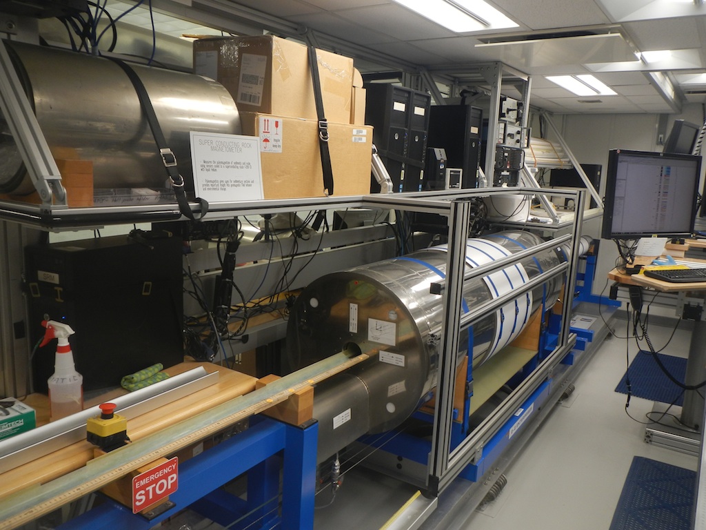
This is the superconducting rock magnetometer, or SRM. We use it to measure the record of Earth’s past magnetic field in split cores (“section halves”) [3]. Everybody likes to say “superconducting rock magnetometer” because it makes you sound cool. But it is a mouthful. We sometimes call it the silver bullet. But usually we just call it the SRM (“ess-are-emm”). We used to have one like it in grad school. We named her Flo.

At the heart of the SRM are three rings made of superconducting wire. These are part of very precise magnetic field sensors called superconducting quantum interference devices, or SQUIDs. We have the other kind of squid out here, too. They are good on the barbecue.
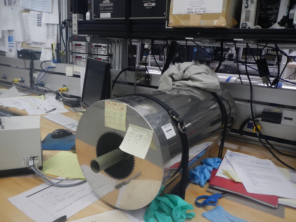
While this looks like the SRM’s little brother, it’s actually a different kind of device. This is the Dtech D-2000 alternating field demagnetizer. Samples that have had their magnetic records partially obscured by big magnetic fields from the drilling process (or by years of growing iron minerals at the bottom of the ocean) need to have those layers of extra magnetic grime scrubbed off by this machine. It works kind of like those old VHS tape erasers, but it’s a lot more precise. It also beeps VERY LOUD.
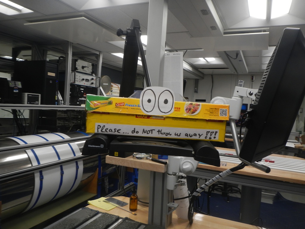
We love plastic wrap in the core lab. We use it to make a nice flat surface for the SHMSL measurements, and to keep the sand and mud from cores out of our magnetometer. We wrap cores in plastic after we’re done analyzing or describing them. Hendrik, a sedimentologist, loves the boxes, too. He was very disappointed that other people kept throwing them away. Some people here think that you can wrap a core faster without the box. Hendrik disagrees. So there was a wrap-off between Hendrik and another sedimentologist. I don’t know who won. I’m agnostic about the boxes. But I do like to keep my magnetometer clean.
[1] In case you are just starting to read this blog, this post is part of my series of posts from the JOIDES Resolution, where I am participating in IODP Expedition 354 to study turbidites on the Bengal Fan.
[2] The optical sensor on the SHMSL is very similar to one that we have in the physics teaching lab at UW Tacoma. You will use it if you take Physics 3. It measures the visible and near-infrared spectrum of light. Magnetic susceptibility – “mag sus” around here – is a measurement of how much magnetic material is in a sediment core. The susceptibility meter applies a very weak magnetic field to the core, and measures the change in the sediment’s magnetization. We have one like it (and a track system for cores) in the Environmental Geology lab at UW Tacoma. Sorry, no SHMSL, though.
[3] Previous posts about the basics of Earth’s magnetic field are here, here, and here. Watch this blog for more about how we use the geomagnetic polarity time scale, or GPTS, to figure out the age of rocks – coming soon!
]]>
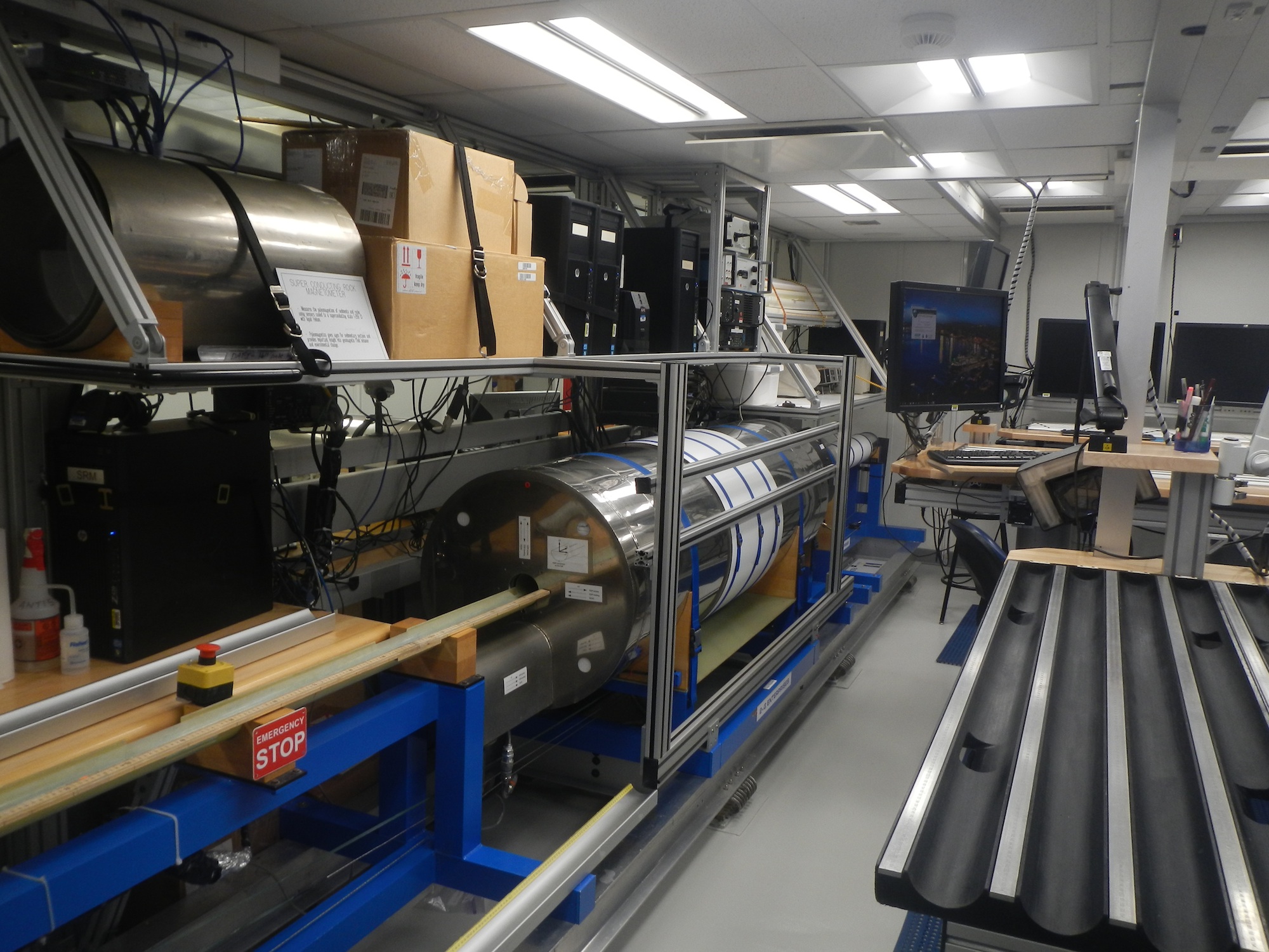 If you can’t see the sign in the photo, this is the superconducting rock magnetometer (SRM) on the JOIDES Resolution. We use it to measure the record of Earth’s ancient magnetic field in rocks and sediments. Right now, we’re running sections of marine sediment cores through the machine. The SRM tells us what direction your compass would have pointed if you were standing here hundreds of thousands – or even millions – of years ago.
Muck in the oceans builds up, layer upon layer, so that older mud eventually gets covered with younger stuff. If you look closely at the muck, you’d see it was composed of lots of tiny particles. These are pieces of clay, silt, and sand formed from the detritus of eroded mountain ranges, the decaying bodies and shells of tiny fossil creatures, dust from the air, tiny crystals that form in the oceans, and even microscopic meteorites. Some of those particles are magnetic. For the most part, those contain the magnetic iron oxide magnetite [1], which can be part of the dregs of continental erosion, or it can be made by bacteria in the ocean, or by a number of other things. As the tiny magnetic particles fall through the water, they turn so that they are magnetized in line with Earth’s magnetic field – just like little compasses [2]. After they fall into the sediment accumulating on the seafloor, the magnetic particles get buried, “locked” in position by the other particles surrounding them. If Earth’s magnetic field switches polarity, the “tiny compasses” in new sediment being deposited will align with Earth’s new magnetic field, but the ones already locked in the sediment will stay as they were.
At least, that’s how the typical story goes about how sediment records the direction of Earth’s magnetic field. In reality, it’s not so simple. For one thing, all kinds of creatures live in the sediment – like whoever lived in this burrow:
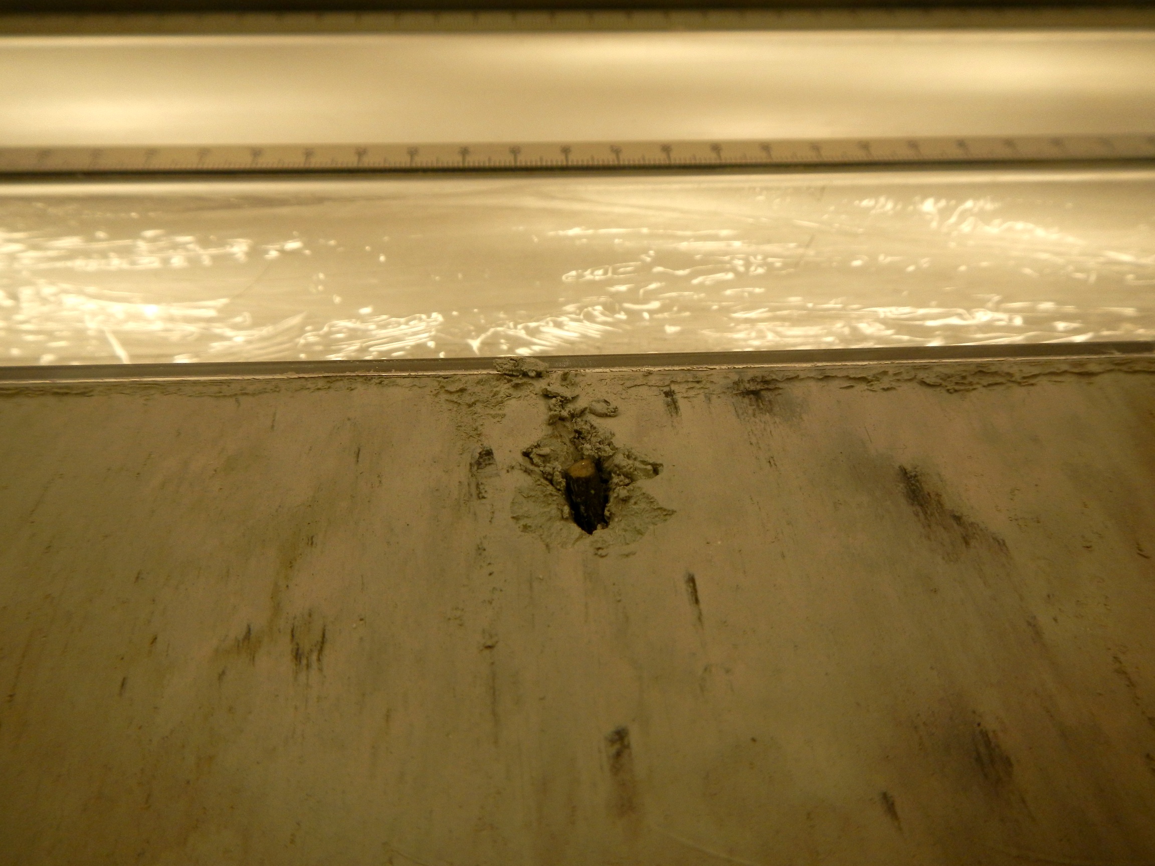
This sediment core is actually full of fossil burrows. But sediments full of burrows can record Earth’s magnetic field just fine. We think it might be because the creatures burrowing in the sediment stir up the muck just enough that it settles back in line with Earth’s magnetic field again. It’s just that the sediment “locks in” the record of the magnetic field after the burrows themselves get buried. That seems reasonable until you realize that this burrow and others like it did not record a magnetic field in the same direction as the sediment around it [3]. This burrow is filled with pyrite, which, though iron-bearing, is not itself magnetic in the same way as magnetite [4]. Some geologists think that something happened to make new magnetic materials form or old ones dissolve around burrows like this one.
To make things even more complex, the area we are looking at on the Bengal Fan was not formed by sediments settling out in quiet water. Instead, much of the sand and mud deposited here was dumped very quickly from places close to land [5]. Do the magnetic particles in these tremendous currents full of churning sand and mud even have time to be pulled by Earth’s magnetic field, or are the forces in the currents too great? It looks like, at least in the muddy parts of deposits like the ones we’re studying, the sediment does keep a mostly faithful record of Earth’s magnetic field.
In the end, the story we tell about how sediments become magnetized is probably fundamentally OK, but there are parts of it we still don’t fully understand. Those parts of the story we’re still curious about are what keep us doing science!
[1] Magnetite is Fe3O4. To a certain extent, hematite (Fe2O3) and goethite (FeOOH) can also be incorporated into marine sediments, along with other magnetic minerals that can grow there.
[2] Unlike in igneous rocks, where the magnetic minerals “lock in” a record of Earth’s magnetic mineral as they cool. The minerals in igneous rocks DO NOT move.
[3] See Abrajevitch, A., Van Der Voo, R., and Rea, D., 2009. Variations in abundances of goethite and hematite in Bengal Fan sediments: Climatic vs. diagenetic signals, Marine Geology 267:191-206.
[4] Pyrite is paramagnetic, meaning that it can be magnetized only in the presence of a magnetic field, not after the field is gone; magnetite is ferromagnetic, meaning that it can be permanently magnetized.
[5]This is called a turbidity current, and the sand and mud deposits it leaves behind are called turbidites.
]]>

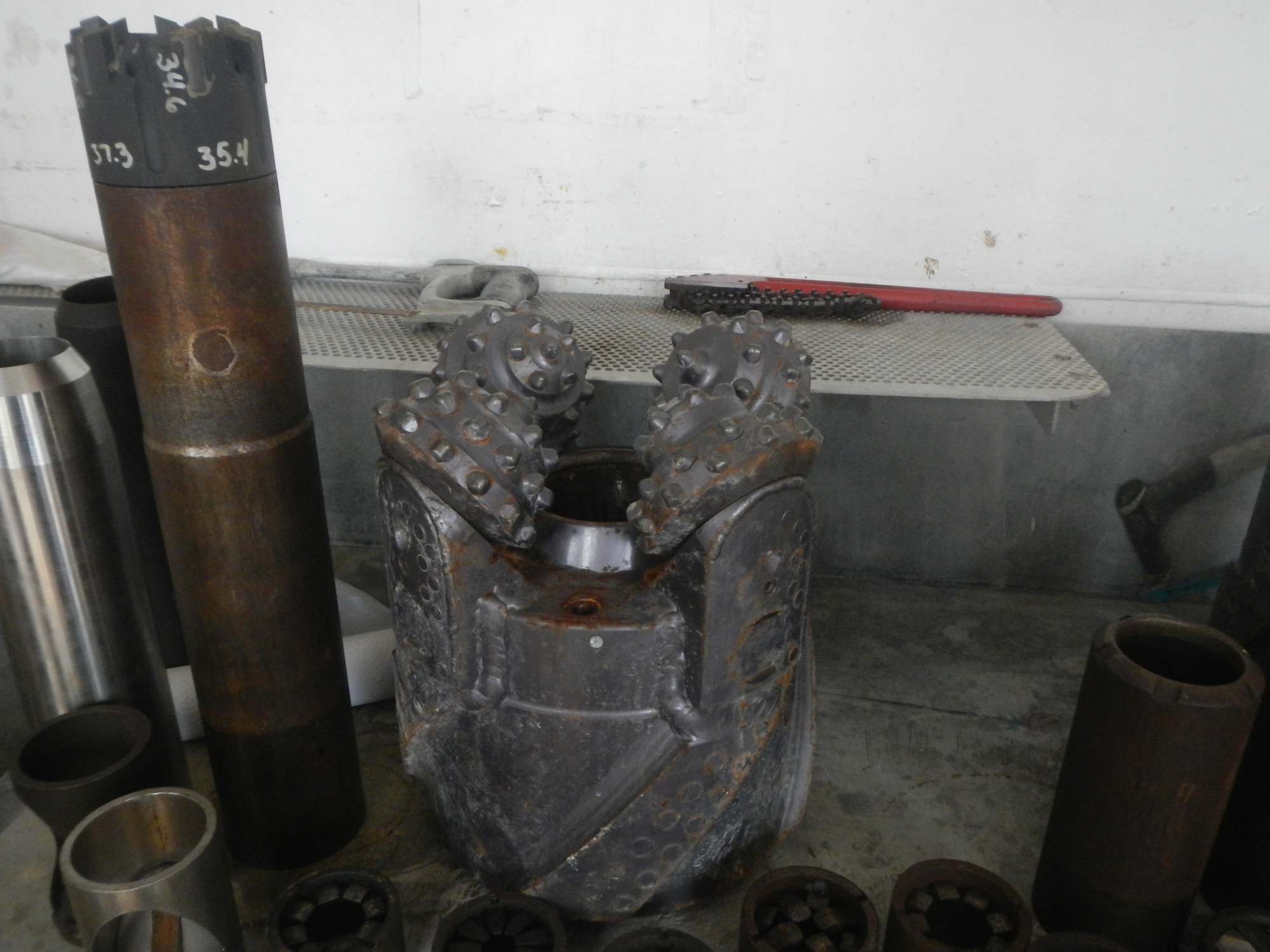
The tower-like structure on the JR is where a lot of the drilling apparatus sits. The drill parts are lowered to the seafloor through a hole in the bottom of the ship – the Moon Pool (no photos of that yet: I can’t go down there).
The drill itself consists of a drill bit, inside of which sits a core barrel. The core barrel sits in the middle of the drill bit. Inside the core barrel is a device that lets sediment in, but not out (the core catcher) and a device to measure temperature. The whole apparatus is lowered down at the end of a drill pipe (an actual pipe), inside of which is a plastic tube (the core liner) that will hold the rock or sediment when we bring it up . Some weights are fitted to the pipe to get it to sit still on the seafloor.
If we are coring sediment, as we will be doing for much of this expedition, we use a device called an Advanced Piston Corer (APC) that punches 27 meters at a time into the sediment, pushed by both gravity and pressurized seawater (or sometimes mud). The APC and the core liner are pulled up out of the drill pipe, the core and liner removed, and the whole thing reloaded for the next 27 meters of coring. Meanwhile, the drill bit spins around, grinding down 27 meters until it gets to the bottom of the hole that the APC made. Then we repeat the process until we get to a couple of hundred meters below the seafloor, where the sediment is too hard for the APC.
There are two reasons we want to use an APC on the sediment here. First, APCs tend to recover a lot of sediment (other kinds of core barrels can break up the sediment, and tend to lose about half of it on the way down). Second, and just as important for us paleomagnetists, we can find the cores’ orientation using a compass-like device attached to the APC drill pipe. This is crucial if we need to know the direction in which the sediment of the Bengal Fan got magnetized: if the core turned around as it came out of the seafloor, we would never know if parts of it were magnetized in a different direction than Earth’s present magnetic field, or if they were just turned around during coring.
We will also be using the XCB on this expedition. The XCB is the Extended Core Barrel, a rotating core device that can cut more solid sediment. The XCB gets less recovery, and the core it takes can’t be oriented.
]]>