The Lollipop war goes back to 1789! But it did not start in earnest until the great depression. Here is the most recent installment (mp3 and transcript):


The Lollipop war goes back to 1789! But it did not start in earnest until the great depression. Here is the most recent installment (mp3 and transcript):
Soros and Sinn weigh in on European Policy Options.
It all seems so black and white: Germany shoulders a greater share of the adjustment, and/or a price adjustment in crisis countries is inevitable. Note that the adjustment will either be an internal devaluation (reduction of prices/wages without a change in the exchange rate) or through an external devaluation (countries exiting the Euro, effectively leaving a fixed exchange rate regime, and depreciate their (new domestic) currencies).
There is also an interesting historical parallel. In The Economic Consequences of the Peace (1919), Keynes argued that Germany's war debt should be largely forgiven. He thought the absence of a German recovery would stifle the economic (and political) recovery of all of Europe. As an advisor to the British Government at the Verailles Conference he argued that German reparations should be limited to £2,000 million. This was less than what Britain owed the US in war loans! Nevertheless he had the audacity to suggest that a general forgiveness of war debts would benefit Britain. Certainly the German transgressions had been more objectionable than the Greek, Cypriot, Irish, Portuguise goverments in the early 2000s.

Econbrowser has a great post on interest-forward rates, and monetary tightening
The Federal Reserve has been trying hard to communicate that it intends to keep short-term interest rates low for quite some time. The market seems to have embraced the message.
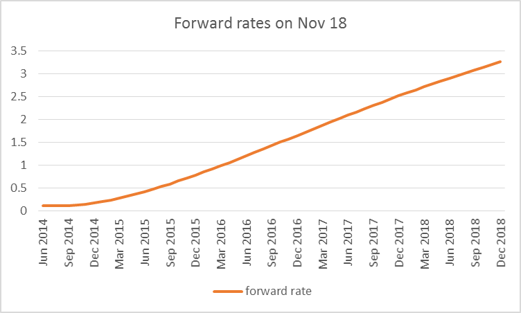
One way to summarize the yields on securities with different maturities is with the forward curve. Suppose that today I sold $1000 worth of a bond that I’ll have to pay back with interest 365 days from now and simultaneously bought $1000 worth of a bond that will pay me back with interest 366 days from now. That would leave me on net owing nothing and receiving nothing for the next year, paying out some money 365 days from now, and getting my money back with interest 366 days from now. In effect, I’ve used today’s interest rates to lock in the return on a one-day security I plan to purchase 365 days from today. The return I could get from that transaction is known as today’s 365-day forward rate.
You can’t usually buy a 366-day bond, but you can fit a smooth function to the yields on whatever bonds you can buy to get an estimate of the 365-day and 366-day interest rate, from which you can calculate the 365-day forward rate, and indeed could calculate the n-day forward rate for any value of n you might be interested in. A paper by Gurkaynak, Sack, and Wright developed a simple way to do that. You can download their summary of the yield curve for any historical date going back to 1961.
I’ve used their data (along with equation (21) in their paper) to calculate what forward rates looked like as of November 18. Their approximation is designed for the longer end of the yield curve, and the very near forward rates you’d calculate from their formula have trouble coping with the zero lower bound. For this reason, I start the graph below with the 6-month forward rate. The date in the future at which I would earn my one-day yield is plotted on the horizontal axis, and the yield at an annual rate is on the vertical axis. The forward curve implies overnight rates that remain below 25 basis points through the end of 2014, and only rise very slowly after that, with the rate still below 2.5% until the end of 2017.
 |
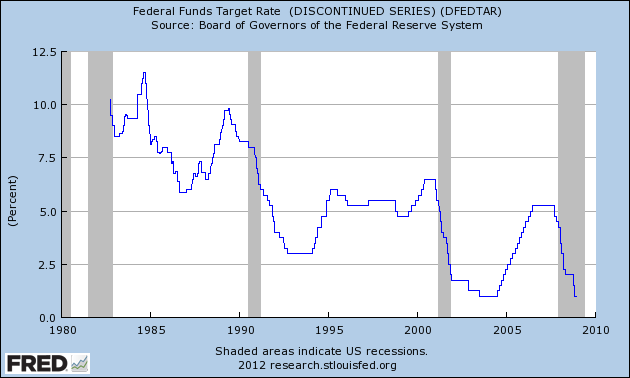
It’s interesting to compare that gradual slope with the actual historical path of short-term interest rates, as summarized by the graph below of the fed funds target.
 |
The table below summarizes what happened during the previous 4 episodes of Fed tightening. These lasted for one or two years and resulted in an increase of the overnight rate of between 175 and 425 basis points. During an average tightening episode, the short-term rate went up by 22 basis points per month. That compares with an average increase of 6 basis points per month implied by the forward curve for a monetary tightening beginning in 2015.
| START | END | CHANGE IN TARGET | CHANGE PER MONTH
|
|---|---|---|---|
| Mar 29, 1988 | Feb 24, 1989 | 3.25 | 0.30
|
| Feb 3, 1994 | Feb 1, 1995 | 3.0 | 0.25
|
| Jun 29, 1999 | May 16, 2000 | 1.75 | 0.17
|
| Jun 29, 2004 | Jun 29, 2006 | 4.25 | 0.18 |
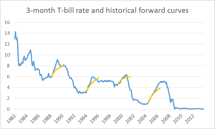
I was curious to go back and see what the forward curve was signaling prior to each of these four episodes. The blue line in the graph below plots the 3-month Tbill rate, while the orange segments show the forward curve looking ahead up to 2 years from the date before the episode began. The forward curve was much more steeply sloped as those episodes began than it is today, and anticipated the Fed tightening fairly well.
 |
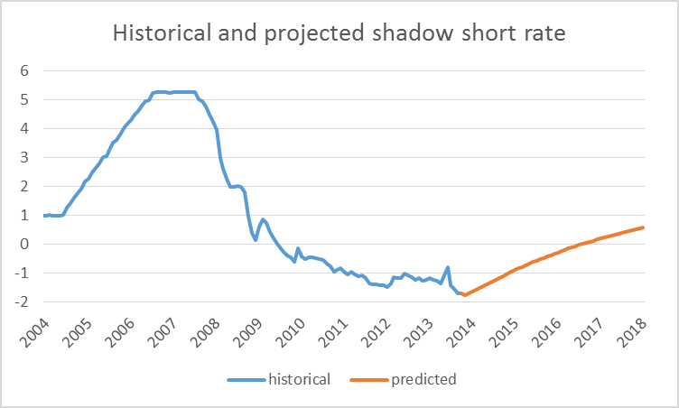
A good deal of economic research has established that there is a risk premium built into these forward rates, particularly as you use them to describe a transaction farther into the future. There are a number of different models people have developed to try to estimate this risk premium. However, the direction of this risk premium suggests that a rational forecast of the short rate would be even lower than the path implied by the forward curve in the first figure above. This for example is the implication of the calculation of the risk premium that comes out of a model of interest rates developed by Wu and Xia (2013) that I described a couple of weeks ago. The Wu-Xia forecast of the shadow rate– a theoretical construct on the basis of which all other interest rates get determined– doesn’t begin to turn positive until September of 2016.
 |
Based on current interest rates, the market thus appears quite convinced that the Fed is indeed not going to begin raising short rates for some time, and that, when it does finally begin to raise rates, it will do so much more slowly than was the case in any of the 4 previous tightenings. Partly this might be judged a success of the Fed’s forward guidance communication efforts, and partly a conclusion that conditions just aren’t going to be strong enough to lead the Fed to want to raise short-term rates for some time. The table below summarizes what the data for unemployment and inflation (as measured by the year-over-year change in the PCE deflator) were like at the start of each of the four historical tightening episodes.
| EPISODE | BEGINNING UNEMPLOYMENT | BEGINNING INFLATION
|
|---|---|---|
| 1988-89 | 5.7 | 3.7
|
| 1994-95 | 6.6 | 2.1
|
| 1999-2000 | 4.3 | 1.6
|
| 2004-2006 | 5.6 | 2.5
|
| AVERAGE | 5.6 | 2.5
|
| Nov 2013 values | 7.3 | 0.9 |
The lowest inflation rate at which the Fed began any of these cycles was 1.6% while the highest unemployment rate was 6.6%. For comparison, the inflation rate currently stands at 0.9% and the unemployment rate at 7.3%. In its most recent policy statement, the FOMC said that it “currently anticipates that this exceptionally low range for the federal funds rate will be appropriate at least as long as the unemployment rate remains above 6-1/2 percent, inflation between one and two years ahead is projected to be no more than a half percentage point above the Committee’s 2 percent longer-run goal, and longer-term inflation expectations continue to be well anchored.” The Survey of Professional Forecasters is anticipating that the unemployment rate won’t be down to 6.6% until 2015, at which time PCE inflation will still only be 2.0%.
It is possible that the Fed will announce a slowdown in the rate of large-scale asset purchases sometime soon, which could affect the long end of the yield curve. But the market is pricing in little risk of a significant move in short rates any time soon. Some might count this as a success of the Fed’s communication strategies. But it could also be interpreted as a market consensus that robust growth for the U.S. economy is not coming any time soon.
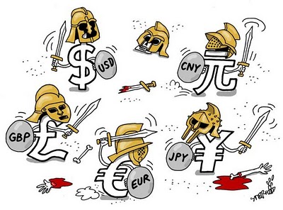
The term "competitive devaluations" or "beggar-thy-neighbor" policies refer to monetary policy designed to lower the exchange rate to increase exports and growth (see IE CH 19). More recently these policies have also been referred to as "currency wars" and even financial "weapons of mass destruction." A recent working paper by the World Bank now equates failures of the gold standard in the 1930s to competitive devaluations. Instead of unilateral devaluations, the World Bank document suggests
The optimal policy response to the Great Depression, in this view, should have been a coordinated, unsterilized devaluation against gold by all countries suffering deflation. In effect, this would have been a coordinated global monetary easing, but without the beggar-thy-neighbor effects on trade.
– How would "coordinated devaluations" across countries have avoided the beggar-thy-neighbor effects
– Can you see any problems with the World Bank's policy prescription?