II.2: Steady-State Simulations
To illustrate how to use Gepasi to simulate steady-state data, let’s set up a two-site random-ordered binding model. Start at the ‘Model Definition’ tab and click on ‘Units’. Choose appropriate units for your system – I usually choose concentration units of μM (uM). Return to the main window and click on ‘Reactions’. Enter the three reactions as shown, clicking ‘Add’ after each one. (The reactions are automatically numbered from R1 onwards.)
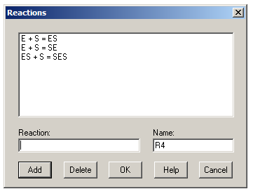
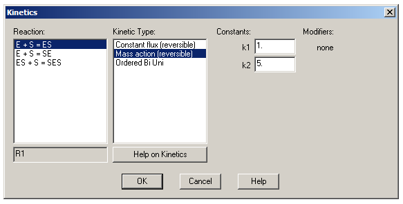
When entering reactions, an equals sign indicates a reversible step and an arrow (typed as ->) indicates an irreversible step. For a steady-state simulation, however, all steps must be reversible. Once you’ve entered your reactions, click OK to return to the Model Definition tab and then click ‘Kinetics’ to define the various KDs in the system. For each reaction, change the kinetic type to ‘Mass action (reversible)’ – this lets you define a kon (k1) and koff (k2) for each reaction. Leave all k1s at the default value of 1 μM-1s-1 and set the value of k2 for each reaction to the desired KD value. (Remember that KD = koff/kon = k2/k1.)
Finally, click on 'Metabolites' to set up the starting concentrations for all of the chemical species in the simulation. For now, change the enzyme concentration to 1 and the substrate concentration to 10. Leave the other concentrations at their default value of 1e-005. (Gepasi can sometimes crash if these values are set to 0.)
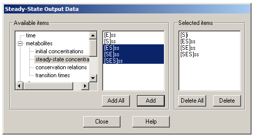
Now that you have set up the model to your satisfaction, go to the Tasks tab. Uncheck the box under ‘Time course’ and leave the ‘Steady state’ box checked. As a default, results from steady state simulations are stored in a plain text file called simresults.ss, but you can change this if you like. You now need to tell Gepasi which specific concentrations to monitor: click the lower ‘Edit’ button. From the list of variables in the left pane, go to ‘metabolites’ and then to ‘initial concentrations’. Click [S]i and then click Add – this initial substrate concentration will serve as the independent variable for plotting later on. Then go to ‘steady-state concentrations’, click on [ES]ss, [SE]ss and [SES]ss and click Add.
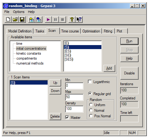
We want to plot the concentrations of the various enzyme-substrate complexes as a function of initial substrate concentration. Return to the main window and switch to the ‘Scan’ tab. Click ‘Enable’, and then choose ‘initial concentrations’ and then [S]i. Click Add, set Min to 0 and Max to five or ten times the highest k2 value you entered in Model Definition – this will ensure the simulated curves will reach saturation. Set Density (the number of points on the plot) to at least 50, and then click ‘Run’ (or the play button on the toolbar) to perform the simulation.
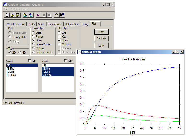
Finally, go to the ‘Plot’ tab. Ensure that the ‘Steady state’ radio button is check, click on [S]i in the X-axis box, and on [ES]ss, [SE]ss and [SES]ss in the Y-axis box. Click ‘Plot!’, and examine the resulting equilibrium binding curves (a.k.a. ‘isotherms’). Return to Model Definition and alter the k2 values in the Kinetics dialog box, to get a sense for how the various KDs alter the relative abundances of the enzyme-substrate complexes.
You can import the 'simresults.ss' file into a program like Excel or Origin to plot it for publication- or presentation-quality images. Here is a Gepasi file made according to the instructions above - you can save it to your computer and open it in Gepasi to compare its results to yours..