1-dimensional acoustics

One-dimensional acoustics

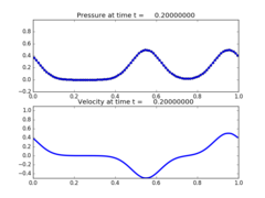
Solve the (linear) acoustics equations:

\[\begin{split}p_t + K u_x & = 0 \\ u_t + p_x / \rho & = 0.\end{split}\]

Here p is the pressure, u is the velocity, K is the bulk modulus, and \(\rho\) is the density.

The initial condition is a Gaussian and the boundary conditions are periodic. The final solution is identical to the initial data because both waves have crossed the domain exactly once.

Output:

Source:

#!/usr/bin/env python
# encoding: utf-8

r"""
One-dimensional acoustics
=========================

Solve the (linear) acoustics equations:

.. math:: 
    p_t + K u_x & = 0 \\ 
    u_t + p_x / \rho & = 0.

Here p is the pressure, u is the velocity, K is the bulk modulus,
and :math:`\rho` is the density.

The initial condition is a Gaussian and the boundary conditions are periodic.
The final solution is identical to the initial data because both waves have
crossed the domain exactly once.
"""
from __future__ import absolute_import
from numpy import sqrt, exp, cos
from clawpack import riemann
    
def setup(use_petsc=False, kernel_language='Fortran', solver_type='classic', outdir='./_output', ptwise=False, \
        weno_order=5, time_integrator='SSP104', disable_output=False):

    if use_petsc:
        import clawpack.petclaw as pyclaw
    else:
        from clawpack import pyclaw

    if kernel_language == 'Fortran':
        if ptwise:
            riemann_solver = riemann.acoustics_1D_ptwise
        else:
            riemann_solver = riemann.acoustics_1D

    elif kernel_language=='Python': 
        riemann_solver = riemann.acoustics_1D_py.acoustics_1D

    if solver_type=='classic':
        solver = pyclaw.ClawSolver1D(riemann_solver)
        solver.limiters = pyclaw.limiters.tvd.MC
    elif solver_type=='sharpclaw':
        solver = pyclaw.SharpClawSolver1D(riemann_solver)
        solver.weno_order=weno_order
        solver.time_integrator=time_integrator
        if time_integrator == 'SSPLMMk3':
            solver.lmm_steps = 4
    else: raise Exception('Unrecognized value of solver_type.')

    solver.kernel_language=kernel_language

    x = pyclaw.Dimension(0.0,1.0,100,name='x')
    domain = pyclaw.Domain(x)
    num_eqn = 2
    state = pyclaw.State(domain,num_eqn)

    solver.bc_lower[0] = pyclaw.BC.periodic
    solver.bc_upper[0] = pyclaw.BC.periodic

    rho  = 1.0 # Material density
    bulk = 1.0 # Material bulk modulus

    state.problem_data['rho']=rho
    state.problem_data['bulk']=bulk
    state.problem_data['zz']=sqrt(rho*bulk) # Impedance
    state.problem_data['cc']=sqrt(bulk/rho) # Sound speed
 
    xc=domain.grid.x.centers
    beta=100; gamma=0; x0=0.75
    state.q[0,:] = exp(-beta * (xc-x0)**2) * cos(gamma * (xc - x0))
    state.q[1,:] = 0.

    solver.dt_initial=domain.grid.delta[0]/state.problem_data['cc']*0.1

    claw = pyclaw.Controller()
    claw.solution = pyclaw.Solution(state,domain)
    claw.solver = solver
    claw.outdir = outdir
    claw.keep_copy = True
    claw.num_output_times = 10
    if disable_output:
        claw.output_format = None
    claw.tfinal = 1.0
    claw.setplot = setplot

    return claw


def setplot(plotdata):
    """ 
    Specify what is to be plotted at each frame.
    Input:  plotdata, an instance of visclaw.data.ClawPlotData.
    Output: a modified version of plotdata.
    """ 
    plotdata.clearfigures()  # clear any old figures,axes,items data

    # Figure for pressure
    plotfigure = plotdata.new_plotfigure(name='Pressure', figno=1)

    # Set up for axes in this figure:
    plotaxes = plotfigure.new_plotaxes()
    plotaxes.axescmd = 'subplot(211)'
    plotaxes.ylimits = [-.2,1.0]
    plotaxes.title = 'Pressure'

    # Set up for item on these axes:
    plotitem = plotaxes.new_plotitem(plot_type='1d_plot')
    plotitem.plot_var = 0
    plotitem.plotstyle = '-o'
    plotitem.color = 'b'
    plotitem.kwargs = {'linewidth':2,'markersize':5}
    
    # Set up for axes in this figure:
    plotaxes = plotfigure.new_plotaxes()
    plotaxes.axescmd = 'subplot(212)'
    plotaxes.xlimits = 'auto'
    plotaxes.ylimits = [-.5,1.1]
    plotaxes.title = 'Velocity'

    # Set up for item on these axes:
    plotitem = plotaxes.new_plotitem(plot_type='1d_plot')
    plotitem.plot_var = 1
    plotitem.plotstyle = '-'
    plotitem.color = 'b'
    plotitem.kwargs = {'linewidth':3,'markersize':5}
    
    return plotdata


def run_and_plot(**kwargs):
    claw = setup(kwargs)
    claw.run()
    from clawpack.pyclaw import plot
    plot.interactive_plot(setplot=setplot)

if __name__=="__main__":
    from clawpack.pyclaw.util import run_app_from_main
    output = run_app_from_main(setup,setplot)