II.4 Fitting Simulations to Experimental Data
First, letĺs try to fit equilibrium binding models to experimental data. To do this in Gepasi, we need to do two things: to define scaling factors that relate the concentrations of various species to an observed experimental signal, and to define functions representing the observed signal that depend on the scaling factors and on the specific concentrations.
Returning to the two-site random-ordered equilibrium binding model we constructed earlier, let us assume that there is an experimental signal to which ES and SES contribute to different degrees. We need to add two scaling factors, one for each of these species. Confusingly, scaling factors in Gepasi are entered as metabolites that are not involved in any reactions and whose concentrations are therefore fixed. From the Model Definition tab, go to the Metabolites dialog box and add two metabolites: name them ĹScale1ĺ and ĹScale2ĺ. Set their starting values (ĹInitial Conc.ĺ) to a suitable guess based on your experimental set-up.
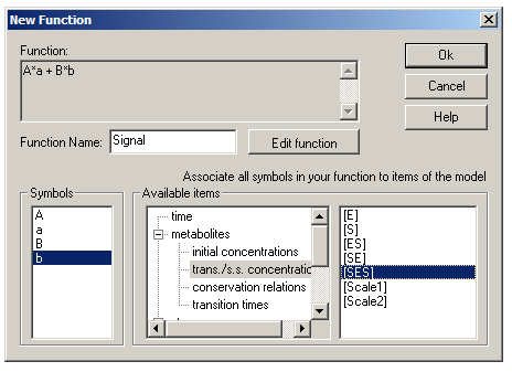
Return to the main window and go to the Functions dialog box. Click the Add button to bring up the New Function box. In Gepasi, functions must be entered as algebraic formula where all symbols are single letters (uppercase or lowercase). These symbols must then be assigned to scaling factors and specific concentrations. Enter the formula ĹA*a + B*bĺ and give it the name ĹSignalĺ. Click ĹAccept Functionĺ, and assign A to Scale1 (under Ĺmetabolitesĺ and Ĺinitial concentrationsĺ), B to Scale2, a to [ES] (under Ĺmetabolitesĺ and Ĺtrans/s.s. concentrationsĺ) and b to [SES].
To keep things simple, letĺs assume that there is no binding cooperativity in the system ľ in other words, the KD for one binding site is not affected by occupancy of the other site. To do this, we need to link the KDs (i.e., koffs) of Reaction 2 (E + S = SE) and Reaction 3 (ES + S = SES). Go to the Links dialog box and add a link. From the ĹAvailable itemsĺ list, go to Ĺkinetic constantsĺ and click R2(k2) ľ this is the off-rate for Reaction 2 ľ and click one of the ĹSetĺ buttons. Now click R3(k2) and click the other Set button. Return to the main window.
A word of warning: if you open the Reactions dialog box and then click OK (even without making any changes), Gepasi will delete any functions and metabolites that you have defined.
Now go to the Tasks tab. Make sure only the ĹSteady stateĺ box is checked, and add [S]i and Signal (under Ĺuser functionsĺ) to the list of variables to be monitored.
Now go to the Fitting tab and click Enable. This is where we choose a data-file (and declare what data are in which columns). Here we also select fitting variables and a fitting algorithm.
Gepasi requires data in plain text files, with independent variable(s) in the leftmost columns and data (user functions) in the rightmost columns. There should be no other text in the data-file ľ click here for an example. Enter the name of your data-file, and then click the ĹData File Formatĺ box. Use the variable list to declare what data are present in your file ľ for this example, the data file contains initial substrate concentration in the first column and observed fluorescence signal in the second column. Enter the number of lines of data in your file in the ĹLinesĺ box in the lower right. Make sure that the ĹSteady stateĺ radio button is checked, and also that the ĹSet model to fitted parametersĺ box is checked.

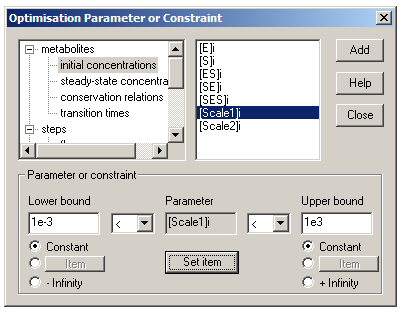
We then need to choose fitting variables for this system ľ in this case, we have two KDs (for Reactions 1 and 2) and two scaling factors. For each fitting variable, click the ĹAdd globalĺ button to bring up the ĹOptimisation Parameter or Constraintĺ dialog. Find each variable in the list (R2(k2) and R3(k2) are under Ĺstepsĺ and Ĺkinetic constantsĺ; Scale1 and Scale2 are under Ĺmetabolitesĺ and Ĺinitial concentrationsĺ). Click ĹSet itemĺ, so that the variable appears in the box labeled ĹParameterĺ. Set bounds for each parameter ľ for both upper and lower bounds, click the ĹConstantĺ radio button, and then enter the bounds. As a rule of thumb, choose upper and lower bounds three orders of magnitude larger and smaller, respectively, than your best guesses.
Once thatĺs done, you need to choose a fitting algorithm from the ĹMethodĺ drop-down list and perform the fit by clicking ĹRunĺ. Levenberg-Marquadt is a powerful and general algorithm used by programs like Origin and Graphpad Prism, but it can get stuck in local minima far away from the optimal solution. Another good choice is the Nelder-Mead (simplex) algorithm, which will reliably avoid local minima and is very quick at going from a poor fit to a reasonably-good fit, but it is quite slow at going from a reasonably-good fit to the true optimal solution. A good strategy is to use both these algorithms in combination: start with Nelder-Mead, and run it until the χ2 (ĹSum of sq.ĺ) value is changing slowly or barely at all. Then click ĹStopĺ, switch to Levenberg-Marquadt, and run it again until it stops of its own accord. After a successful fit, Gepasi will generate a text file with the name of your simulation that contains the χ2 values from the fit, as well as fitting standard errors and parameter covariance matrix.
You can also switch to the Plot tab, make sure the ĹFittingĺ radio button is checked, and plot your independent variable on the X-axis against the experimental data (Signal), fitted modeled data (Signal*), and residuals (E(Signal)).

The Gepasi file used to generate the figures above is available here.
When it comes to fitting turnover kinetics from data of product formed after a specific time interval, your data-file must have the time at which you quenched your reaction in the first column, substrate and/or inhibitor concentrations in the next column(s), and product formed in nmol as the last column. Set up a time course simulation as previously described, and perform the fit as described above. The fitting parameters will include the kcats and KMs of the system. Note that when using kinetic simulations, you do not need to be overly stringent when limiting yourself to data from the linear regime of product curves ľ kinetic simulations automatically correct for substrate depletion effects and the consequent non-linearity of product formation curves.