II.3: Simulating Turnover Kinetics
Now let’s use Gepasi to simulate the same random-ordered turnover model we solved earlier using analytical equations. We will produce both product-time and velocity-substrate plots for this system.
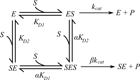
In addition to the three reversible binding steps, add two reactions (in the Reactions dialog box) for the two catalytically active species ES and SES.

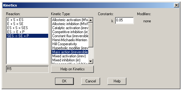
In the metabolites, ensure that starting enzyme and substrate concentrations are set at 1 and 10 respectively, and leave the other species’ concentrations at 1e-005. In the Kinetics dialog box, choose the ‘Mass action (irreversible)’ type for both new reactions. The parameter k for each reaction is the kcat for that step. Set the kcats at least ten-fold lower than the koffs for now, so that our model shows rapid-equilibrium kinetics.
Now in the Tasks tab, make sure that ‘Time course’ is checked and ‘Steady state’ is not. By default, time course data are stored in a plain text file called simresults.dyn by default. Click on the ‘Edit’ button to select what data will be stored in this file: from the variable list, choose ‘time’ and then ‘time’ again. Under ‘metabolites’, choose ‘initial concentrations’ and then [S]i; then choose ‘transient concentrations’ and then [P]t. Returning to the main window, the ‘End time’ is the length of the simulation in seconds and ‘Points’ is the number of time points for which data will be recorded and plotted. For now, send ‘End time’ to 60 seconds, and ‘Points’ to 50.

Go to the Scan tab, and add the initial substrate concentration [S]i to the ‘Scan items’ list. Click on [S]i in the list and set Min to 0 and Max to five or ten times your calculated KM. Set density to 20. Run the simulation, and then go to the Plot tab. Once the ‘Time course’ radio button is selected, choose ‘time’ for the X-axis and ‘[P]t’ in the Y-axis. Click plot, and observe how the product curves appear mostly linear, and how their slopes approach a limiting value. Try extending the simulation to longer timescales, and get a sense of how these curves deviate from linearity. See how different kcats and KMs alter these curves.

Now return to the Tasks tab. To plot a velocity-substrate graph, we want to know the product levels after a short time interval – if we are still in the regime of linear product curves, then the velocity is directly proportional to the amount of product formed. So set the End Time to 10 (seconds), and the Points to 1. Now the resulting data file will contain only initial and final values for the specific concentrations you’ve chosen. In the Scan tab, set Points to 50. Run the simulation again, and return to the Plot tab. Choose [S]i for the X-axis and [P]t for the Y-axis, and choose ‘Points’ under ‘Data Style’. See how this plot is affected by different kcats and KMs, and by different values for the simulation’s End Time.

Again, here's a copy of the Gepasi file used to generate the figures above.