As part of the Cascadia CoPes Hub project, a new set of 36 ground motions have been computed using 3D simulations, archived on Design Safe at Dunham et al. (2025).
The surface deformation from these ground motions can be used as sources for tsunami simulations. Several different versions of these have been computed, including for the full time-dependent kinematic rupture, but also static displacements for “instantaneous” tsunami generation. The development of these sources and their potential use for tsunami modeling is described in this paper: Dunham et al. (2025).
Recently a modified set of events has also been generated that we feel are better to use for tsunami modeling. These 36 events are closely related to the original events but without the high-frequency subevents that are used to model and match expected shaking at high-frequencies (> 1Hz), since these were found to have a significant impact on the low-frequency and permanent deformation near the coast (which is critical to properly model in tsunami simulations). We also modified the downdip extent of slip for one branch of the logic tree so that our scenarios collectively better matched the range of expected subsidence from paleoseismic data along the coast. For these new events, full 3D seismic simulations were not performed. Instead the Okada elastic half-space model was used to approximate the surface deformation (including a kinematic version, as described below in Kinematic Okada (KinOkada) deformations.).
To use these ground motions in simulations on TACC, see Shared data files on TACC.
Logic Tree
The names of the 36 events are based on a logic tree that follows the National Seismic Hazard Model (NSHM) logic tree for Cascadia megathrust earthquakes where possible, which includes the following weights for the downdip limits: Deep: 0.2, Middle: 0.5, Shallow: 0.3 (Petersen et al. (2014); Petersen et al. (2024)). The weights for the buried (0.75) and frontal thrust (0.25) are based on the logic tree developed by the USGS Powell Center Tsunami Sources Working Group (Sypus and Wang, 2024). Within each of these 6 branches there are 6 earthquake scenarios that have equal weights, since both the slip distribution and magnitude-area relationship branches are equally weighted. For the tsunami sources, we modified the middle downdip limit of slip from the NSHM so that it better matched paleoseismic subsidence estimates along the coast. The original middle downdip limit of slip is based on the 1 cm/yr locking contour from a combination of the McCaffrey et al. (2013) and Burgettes et al. (2009) locking models. To modify it, we took the 1 cm/yr locking contour from Li et al. (2018) which is very comparable to the NSHM with slightly deeper slip in central Cascadia, leading to a better overall fit to paleoseismic estimates of subsidence.
This figure shows the structure of the logic tree and the assumptions and weights for each branch (click to view):
Logic Tree Version 1

Here’s a more tree-like view of the logic tree in which only the top- and bottom-most branches are displayed in full:
Logic Tree Version 2
The table below shows a list of all 36 sources from the logic tree,
with their associated short names (e.g. buried-locking-str10-deep
is abbreviated BL10D) and the weight of each obtained as the product of
the weights from the logic tree branches leading to each leaf.
Note that these weights could potentially be used as conditional probabilities, i.e. assuming that one of these 36 events happens, the weight can be viewed as the probability of this event. To compute annual probabilities of occurrence, as needed for PTHA, one could assign a probability such as for the occurrence of “some such CSZ event”, and then multiply each of the weights below by this value . A recurrence rate of 1/526 for full-margin Cascadia earthquakes is suggested by the National Seismic Hazard Model that this logic tree is based on (Frankel et al., 2015).
List of 36 sources - names and weights
| event number | event | long name | weight |
|---|---|---|---|
| 1 | BL10D | buried-locking-str10-deep | 0.03750 |
| 2 | BL10M | buried-locking-str10-middle | 0.06250 |
| 3 | BL10S | buried-locking-str10-shallow | 0.02500 |
| 4 | BL13D | buried-locking-mur13-deep | 0.03750 |
| 5 | BL13M | buried-locking-mur13-middle | 0.06250 |
| 6 | BL13S | buried-locking-mur13-shallow | 0.02500 |
| 7 | BL16D | buried-locking-skl16-deep | 0.03750 |
| 8 | BL16M | buried-locking-skl16-middle | 0.06250 |
| 9 | BL16S | buried-locking-skl16-shallow | 0.02500 |
| 10 | BR10D | buried-random-str10-deep | 0.03750 |
| 11 | BR10M | buried-random-str10-middle | 0.06250 |
| 12 | BR10S | buried-random-str10-shallow | 0.02500 |
| 13 | BR13D | buried-random-mur13-deep | 0.03750 |
| 14 | BR13M | buried-random-mur13-middle | 0.06250 |
| 15 | BR13S | buried-random-mur13-shallow | 0.02500 |
| 16 | BR16D | buried-random-skl16-deep | 0.03750 |
| 17 | BR16M | buried-random-skl16-middle | 0.06250 |
| 18 | BR16S | buried-random-skl16-shallow | 0.02500 |
| 19 | FL10D | ft-locking-str10-deep | 0.01250 |
| 20 | FL10M | ft-locking-str10-middle | 0.02083 |
| 21 | FL10S | ft-locking-str10-shallow | 0.00833 |
| 22 | FL13D | ft-locking-mur13-deep | 0.01250 |
| 23 | FL13M | ft-locking-mur13-middle | 0.02083 |
| 24 | FL13S | ft-locking-mur13-shallow | 0.00833 |
| 25 | FL16D | ft-locking-skl16-deep | 0.01250 |
| 26 | FL16M | ft-locking-skl16-middle | 0.02083 |
| 27 | FL16S | ft-locking-skl16-shallow | 0.00833 |
| 28 | FR10D | ft-random-str10-deep | 0.01250 |
| 29 | FR10M | ft-random-str10-middle | 0.02083 |
| 30 | FR10S | ft-random-str10-shallow | 0.00833 |
| 31 | FR13D | ft-random-mur13-deep | 0.01250 |
| 32 | FR13M | ft-random-mur13-middle | 0.02083 |
| 33 | FR13S | ft-random-mur13-shallow | 0.00833 |
| 34 | FR16D | ft-random-skl16-deep | 0.01250 |
| 35 | FR16M | ft-random-skl16-middle | 0.02083 |
| 36 | FR16S | ft-random-skl16-shallow | 0.00833 |
Kinematic rupture models
These 36 events were defined by first specifying a fault geometry for the Cascadia Subduction Zone megathrust surface (McCrory et al., 2012). For frontal thrust events, we used additional splay fault geometries from Ledeczi et al. (2024) and Lucas et al. (2025) Our fault geometry consists of a large number of triangular subfaults. For each event, several quantities are defined on each of the subfaults, including:
slip: The magnitude of the slip (relative displacement along subfault),
rake: The direction of the slip along the subfault,
rupture time: The time the slip of this subfault starts,
rise time: Determines the time history of the slip on this fault.
For each event, the resulting ground motion can then be determined as described below. This is called a kinematic rupture because the time-dependent slip is specified a priori. (By contrast a dynamic rupture would attempt to model how the slip evolves using fracture mechanics based on presumed stresses within the Earth.)
The slip distribution for each scenario is generated using von Karmon correlation functions where the correlation lengths are chosen to reflect the magnitude of the modeled earthquake based on empirical relationships of global events. We randomly generate the slip distribution for each scenario. For the “locking” branch of the logic tree, we weight a randomly generated slip distribution by interseismic geodetic locking (Li et al., 2018) which allows higher slip in regions of higher locking, which has been seen in other large earthquakes globally.
The earthquake scenarios are developed using what we call a “compound rupture model” where we combine long-period (low-frequency) background slip in the updip portion of the rupture with short-period (high-frequency) subevent slip in the downdip portion of the rupture. These high frequency patches, or subevents, have been observed and modeled for great subduction zone earthquakes globally and are necessary to match expected strong ground motion shaking from these events. The distribution of the background slip is most important for tsunami generation whereas the subevent slip is most important for matching high-frequency, strong shaking. he figure below shows a comparison between the subevent distribution from the 2011 M9.1 Tohoku-Oki earthquake and an example CSZ scenario.
Figure showing subevent distributions

Seismic modeling and earthquake ground motions
The seismic simulation code SPECFEM3D was used to simulate wave propagation in 3-D using a seismic velocity model for Cascadia (Stephenson et al., 2017). This produces synthetic waveforms (i.e., time series) of ground shaking and displacement for each scenario, which were captured at grid points on the Earth surface (at 0 m sea-level).
For the purposes of tsunami modeling, the vertical deformation time series at
each grid point on the Earth surface have been subsampled in space and time to
produce a set of vertical deformations every 10 seconds over the duration
of the earthquake (generally less than 500 seconds).
For the GeoClaw tsunami model, these are stored as dtopo files.
Although initial tsunami simulations were performed using these deformation outputs, we observed that for many events the deformation near the coast was not always consistent with the geologic evidence of subsidence in past tsunami events. Investigation revealed that the subevents that were added to provide realistic high-frequency shaking in the seismic wave forms resulted in artifacts in the vertical deformation that were often particularly large near the coast due to the location of the subevents. While subevents are necessary to model high-frequency energy from these earthquake scenarios, they result in modeling artifacts that impact deformation, and therefore, the tsunami generation.
As a result, a new set of scenarios were developed that correspond
to similar earthquakes but without the subevents (NOSUB). Each of these
36 events has the same magnitude, slip distribution,
and rupture timing as the original event it was
based on, but with slip reassigned from the subevents to the main
rupture. These new NOSUB events do not have the
same high-frequency shaking as the originals, but for tsunami
modeling these high-frequency waves have little effect. They are
better for tsunami modeling since the final vertical displacement
at the end of the earthquake (which is the primary driver of the
tsunami) behaves more realistically along the coast.
Full seismic simulations of the 36 NOSUB events have not been
performed, since these would be computationally expensive and the
full seismic signal is not needed for tsunami modeling. (And these
modified sources would not be useful for seismic hazard assessment
either, since they would be missing the high-frequency contributions
of the subevents). Instead, the sea floor deformations used as the
tsunami model inputs were computed using the approach described
below in Kinematic Okada (KinOkada) deformations.
Okada model of an elastic halfspace
For tsunami modeling, we are primarily interested in low-frequency components of the vertical deformation of the sea floor, and in particular, the final deformation after all the seismic P-waves and S-waves have propagated away. For this reason, tsunami modeling is often based on a single static deformation that is an estimate of the final permanent deformation, without solving for the elastic waves. If we assume the Earth is a homogeneous elastic halfspace with a free surface at the top surface, then it is possible to compute the static deformation of the surface due to slip on a single triangular subfault. This is often called the Okada model for deformation, since formulas for this deformation due to a point source or a rectangular subfault were published in widely cited papers by Y. Okada 1985, 1992. The final static deformation for one of our events can be approximated by using the final slip (at large time) on each subfault, applying the Okada model to each in order to calculate the vertical deformation at each point on a grid specified on the surface, and then summing these up over all subfaults (since this model approximates linear elasticity).
In tsunami modeling, this deformation is often then applied as an
“instantaneous” rupture happening at the initial time of the
simulation. This approach loses all information about the time-dependent
behavior of the kinematic rupture, but since tsunami wave propagation
generally happens on a much slower time scale than the earthquake rupture,
this is often a decent approximation. We have computed a set of
deformations of this nature that we give names like BL10D_instant.
However, we suggest instead using the “KinOkada” versions described next.
Kinematic Okada (KinOkada) deformations
Since many Cascadia CoPes Hub researchers are interested in modeling the combined effect of the earthquake and tsunami, and are interested in the time scales over which these hazards evolve for different events, we have also created a set of deformations that are based on the Okada model but that evolve in time, similar to the original seismic model. This “Kinematic Okada” version is obtained by using the Okada elastic halfspace model to compute the static deformation that results from the specified slip on each subfault, but then we accumulate the global deformation on our surface grid by adding in each such static deformation starting at the time specified by the rupture time for the subfault, and rising smoothly from 0 to the final deformation over the time specified by the rise time of the subfault. This still ignores the propagation of seismic waves and assumes that slip on the fault is instantaneously transferred to static deformation of the surface, but with the time of this transfer governed by the time-dependent kinematic rupture properties of the particular event.
Some animations
This animation shows a comparison of the vertical deformation dZ from
the original seismic model of BL10D and from the KinOkada approximation
to the NOSUB version of the same event:
Animation of BL10D Seismic vs KinOkada vertical deformation
Note in the animation above that the KinOkada deformation evolves in a similar manner to the original, but does not exhibit some of the rectangular-shaped artifacts along the coast seen with the seismic model on the original model with rectangular subevents. In particular, note that some coastal regions in the south that exhibit uplift (red) in the original instead have subsidence (blue) in the KinOkada version without the subevents.
The reason the KinOkada deformation looks much more noisy than the original is due to the fact that the modified source was also prescribed on a much coarser set of subfaults than the original. The original used 350-650K triangular subfaults (with roughly 500 m resolution), which was downsampled to about 8000 subfaults for the KinOkada version. This was done because applying Okada is itself expensive, and again the high-frequency details in the original sources are not so important for the tsunami generation.
The next animation shows (for a different event) the seismic waves propagating away from the fault during the rupture, as computed with the original SPECFEM3D simulation (on the left0), together with the vertical deformation approximated by the KinOkada version (on the right):
Animation of BR13D Seismic waves vs KinOkada deformation
The vertical deformation generates the tsunami, as shown in this animation:
Animation of BR13D Seismic waves vs KinOkada with tsunami waves
The animation above shows only the first 5 minutes after the earthquake rupture starts, by which time the seismic waves are propagating out of the computational domain. The tsunami evolves over a slower time scale, as shown in the next animation over 40 minutes.
Animation of BR13D tsunami waves over 40 minutes
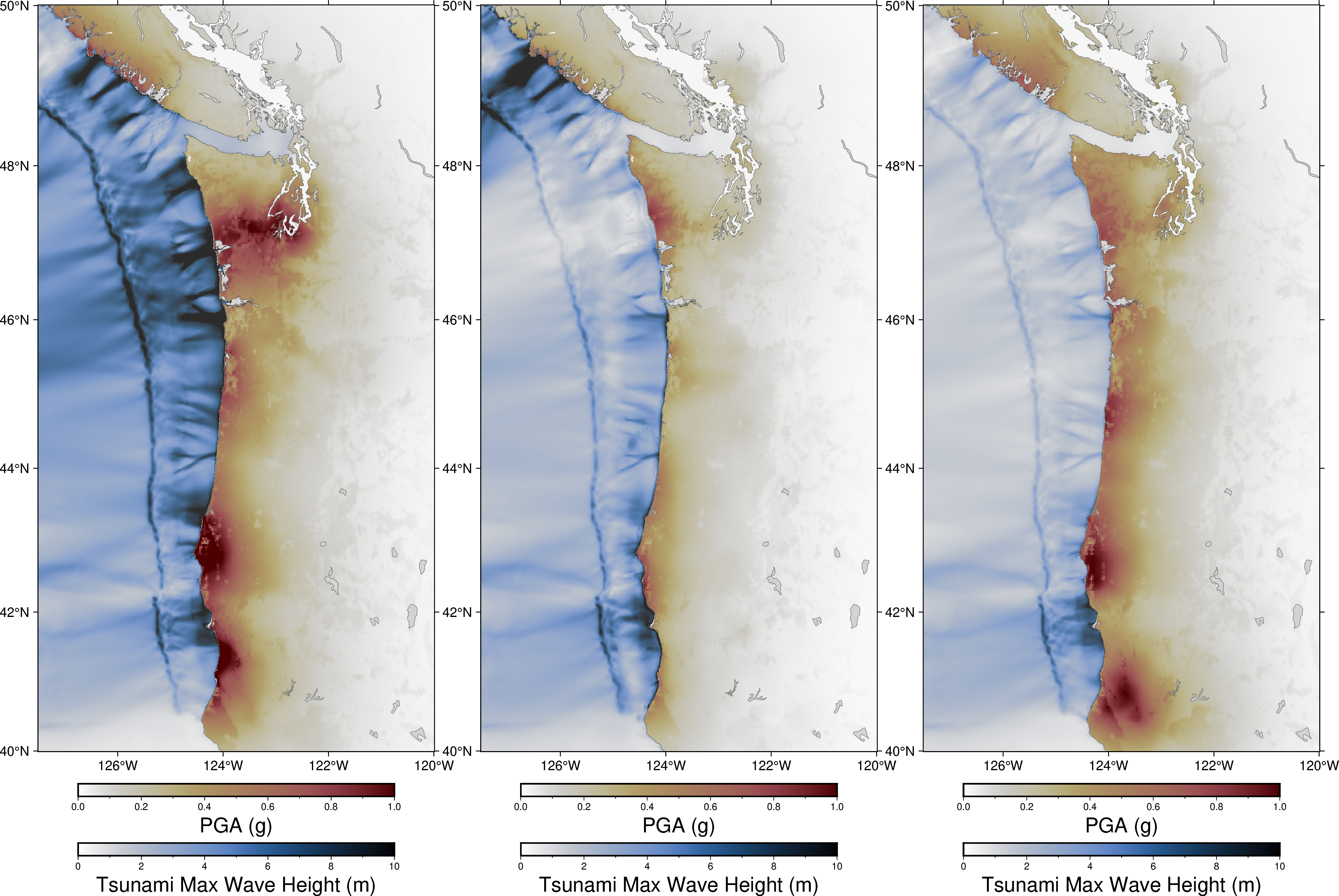
Combining shake maps with tsunami amplitude maps
The figure below shows an earthquake shake map (peak ground acceleration, PGA) onshore with the maximum tsunami amplitude offshore for 3 sample earthquake scenarios.
- Dunham, A., Wirth, E., grant, alex, & Frankel, A. (2025). CSZ Full-Margin Megathrust Earthquake Scenarios. Designsafe-CI. 10.17603/DS2-DQRM-DH11
- Dunham, A. M., Kim, J., Wirth, E., Schmidt, D., LeVeque, R. J., Wei, Y., Adams, L. M., & Pollitz, F. (2025). The Impact of 3D Structure on Coseismic Coastal Land‐Level Change and Tsunami Generation in the Cascadia Subduction Zone. Geophysical Research Letters, 52(24). 10.1029/2025gl117783
- Petersen, M. D., Moschetti, M. P., Powers, P. M., Mueller, C. S., Haller, K. M., Frankel, A. D., Zeng, Y., Rezaeian, S., Harmsen, S. C., Boyd, O. S., Field, E. H., Chen, R., Rukstales, K. S., Luco, N., Wheeler, R. L., Williams, R. A., & Olsen, A. H. (2014). Documentation for the 2014 update of the United States national seismic hazard maps. In Open-File Report. US Geological Survey. 10.3133/ofr20141091
- Petersen, M. D., Shumway, A. M., Powers, P. M., Field, E. H., Moschetti, M. P., Jaiswal, K. S., Milner, K. R., Rezaeian, S., Frankel, A. D., Llenos, A. L., Michael, A. J., Altekruse, J. M., Ahdi, S. K., Withers, K. B., Mueller, C. S., Zeng, Y., Chase, R. E., Salditch, L. M., Luco, N., … Witter, R. C. (2024). The 2023 US 50‐State National Seismic Hazard Model: Overview and implications. Earthquake Spectra, 40(1), 5–88. 10.1177/87552930231215428
- Ledeczi, A., Lucas, M., Tobin, H., Watt, J., & Miller, N. (2024). Late Quaternary Surface Displacements on Accretionary Wedge Splay Faults in the Cascadia Subduction Zone: Implications for Megathrust Rupture. Seismica, 2(4). 10.26443/seismica.v2i4.1158
- Lucas, M. C., Ledeczi, A. M., Tobin, H. J., Carbotte, S. M., Watt, J. T., Han, S., Boston, B., & Jiang, D. (2025). No evidence for an active margin-spanning megasplay fault at the Cascadia Subduction Zone. Seismica, 2(4). 10.26443/seismica.v2i4.1477
- Okada, Y. (1985). Surface deformation due to shear and tensile faults in a half-space. Bull. Seism. Soc. Am., 75, 1135–1154.
- Okada, Y. (1992). Internal deformation due to shear and tensile faults in a half-space. Bull. Seism. Soc. Am., 82, 1018–1040.