LoadGaugesWestportBridges

Load gauge time series from netCDF file¶

Under development for the Cascadia CoPes Hub project, supported by NSF.

This notebook uses a datafile containing gauge time series the 36 ground motions developed for the Cascadia CoPes Hub, at gauge locations near Westport, WA, for a 2-hour simulation using GeoClaw with 1/3 arcsecond resolution on the finest grid level.

This data file can be found from the Design Safe Jupyter Hub in

/home/jupyter/CommunityData/geoclaw/CHTdata/WestportBridges/WestportBridges_gauges_4events_251208.nc

If you have an account on TACC, you can also scp the file from:

username@stampede3.tacc.utexas.edu:/corral/projects/NHERI/community/geoclaw/CHTdata/WestportBridges/WestportBridges_gauges_4events_251208.nc

The gauge locations are on an interactive map that can be created in this notebook.

%matplotlib inline

from pylab import *
import xarray
import os,sys
from pathlib import Path

sys.path.insert(0,'../../src')
import CHTuser

from CHTuser import CHTtools

Read the netCDF file containing all time series¶

Make sure ncfile includes the correct path to the netCDF file with gauge results.

CHTdata = Path('/home/jupyter/CommunityData/geoclaw/CHTdata')  # on Design Safe Jupyter Hub

if not CHTdata.is_dir():
    # Not on Design Safe, hope that there's a local version:
    CHTdata = Path(f'{os.environ['HOME']}/CHTdata')  # local version

print(f'Using path CHTdata = {CHTdata}')

ncfile = Path(CHTdata, 'WestportBridges/WestportBridges_gauges_4events_251208.nc')

Using path CHTdata = /Users/rjl/CHTdata

gauge_x, gauge_y, gauge_t, gauge_vals = CHTtools.read_allgauges_nc(ncfile)

Trying to read /Users/rjl/CHTdata/WestportBridges/WestportBridges_gauges_4events_251208.nc  ...

All gauge output for WestportBridges
Loaded 1441 times from t = 0.0 to 7200.0 sec at 10 gauges
   for 4 events, with qois ['h' 'u' 'v' 'eta' 'level']
print gauge_vals.coords for more info

Examine the data:¶

gauge_vals

Convert to an xarray dataset¶

gauge_vals is one large 4-dimensional array indexed by the quantity of interest qoi as well as by event, gaugeno, and time. For most purposes it’s easiest to convert is to an xarray.Dataset, a collection of DataArray’s split up by the qoi:

ds = gauge_vals.to_dataset(dim='qoi')

ds

print('\nEvents: \n',ds.coords['event'].data)
print('\nGauges: \n',ds.coords['gaugeno'].data)
print(f'\nAt {len(ds.coords['time'])} times up to {array(ds.coords['time']).max()/3600} hours\n')


Events: 
 ['BL10D' 'BL13D' 'BL13M' 'BR13D']

Gauges: 
 [ 62  69  72 234 237 337 423 435 445 446]

At 1441 times up to 2.0 hours

Plot gauge locations¶

Here’s a way to make an interactive folium map showing one or more gauge locations...

def folium_plot_gauge(gaugenos, center=None, zoom_start=13):
    import folium
    import numpy as np

    if not isinstance(gaugenos, (list, tuple, np.ndarray)):
        # If it's not a list, wrap it in one
        gaugenos = [gaugenos]
       
    #tiles = 'OpenStreetMap'  # default tiles
    tiles = 'OpenTopoMap'   # show contours
    
    m = None

    for gaugeno in gaugenos:
 
        xg = gauge_x.sel(gaugeno=gaugeno)
        yg = gauge_y.sel(gaugeno=gaugeno)
        #print(f'Gauge %i is at (%.5f, %.5f)' % (gaugeno, xg, yg))

        if m is None:
            if center is None:
                location=(yg, xg)
            elif isinstance(center,int):
                xgc = gauge_x.sel(gaugeno=center)
                ygc = gauge_y.sel(gaugeno=center)
                location = (ygc, xgc)
            else:
                #assume center is (y,x) location
                location = center
            
            m = folium.Map(location=location, tiles=tiles, zoom_start=zoom_start)
        
        folium.Marker(
            location=[yg,xg],
            #popup = f"<b>Gauge {gaugeno}</b>\n ({xg:.6f},\n{yg:.6f})",
            popup = f"<b>Gauge {gaugeno}</b>\n {yg:.6f}N\n{-xg:.6f}W",
            tooltip="Click for info",
            icon=folium.Icon(color="red")  #, icon="cloud") # Customize the marker's appearance
        ).add_to(m) 
        
    return m

mygaugeno = 234
map = folium_plot_gauge(mygaugeno)  #  argument can be single gauge or list of gauges
print(f'Location of Gauge {mygaugeno}:')
map

Location of Gauge 234:

Make an html file with interactive map showing all gauges:¶

all_gauges = ds.coords['gaugeno'].data
map_with_all_gauges = folium_plot_gauge(all_gauges, center=(46.85,-124), zoom_start=11)
fname = 'WestportBridges_gauges_folium_map.html'
map_with_all_gauges.save(fname)
print('Created ',fname)

# to display the map here, uncomment the next line:
map_with_all_gauges

Created  WestportBridges_gauges_folium_map.html

Adding new qoi’s¶

Now we can refer to ds.h, for example, to get the h variable (rather than having to use gauge_vals.sel(qoi='h').

We can also easily add new quantities of interest to the dataset that are computed from others, e.g. the momentum flux.

ds['momflux'] = ds.h * (ds.u**2 + ds.v**2)

momflux_max = float(ds.momflux.max())
print(f'ds.momflux has shape {ds.momflux.shape}')
print(f'   and the maximum value over all events / gauges /times is {momflux_max:.2f} m^3/s^2')

ds.momflux has shape (1441, 10, 4)
   and the maximum value over all events / gauges /times is 60.42 m^3/s^2

Filtering out coarse-grid values¶

With the AMR strategy now being used, the finest level grids are not added near the gauges until the tsunami is arriving. Plots of the water depth before this time may show non-physical discontinuities at times where the AMR level changed, since on a coarse grid the topography is different and the water depth may be deeper or shallower as a result. (Plotting the surface level eta = h+B, where B is the topography value, would give smoother results at offshore gauges but might show discontinuities at onshore gauges. See this example for more discussion.)

The gauge quantity ds.level contains the AMR level from which the time series data was captured at each time, so we can use this to filter our coarse grid times and define a new variable hfine that is masked at these points and only has data from the finest level:

hfine = ma.masked_where(ds.level != ds.level.max(), ds.h)

ds['hfine'] = (('time','gaugeno','event'),hfine)

Some gauges never had fine grids!¶

For the WestportBridges location, some gauges never got wet and the AMR algorithms never refined around them, so filtering out coareser grids leaves nothing to plot.

Since these gauges are all on dry land, do not do the filter for the plots below...

Select one gauge for one event¶

mygaugeno = 234
myevent = 'BL10D'
xg = gauge_x.sel(gaugeno=mygaugeno)
yg = gauge_y.sel(gaugeno=mygaugeno)
print(f'Gauge {mygaugeno} is at x = {xg:.6f}, y = {yg:.6f}')

Gauge 234 is at x = -124.091920, y = 46.809950

Plot all the data and also the filtered data from the finest AMR level only:¶

hfine = ds.hfine.sel(gaugeno=mygaugeno, event=myevent)
h = ds.h.sel(gaugeno=mygaugeno, event=myevent)
figure(figsize=(10,6))
tminutes = gauge_t / 60.
    
plot(tminutes, h, 'r',label='all data')
plot(tminutes, hfine, 'b',label='finest AMR level')

grid(True)
legend(loc='upper right', framealpha=1)
xlabel('minutes')
ylabel('meters')
title('Water depth at Gauge %i (%.5f, %.5f)\nEvent %s' % (mygaugeno,xg,yg,myevent));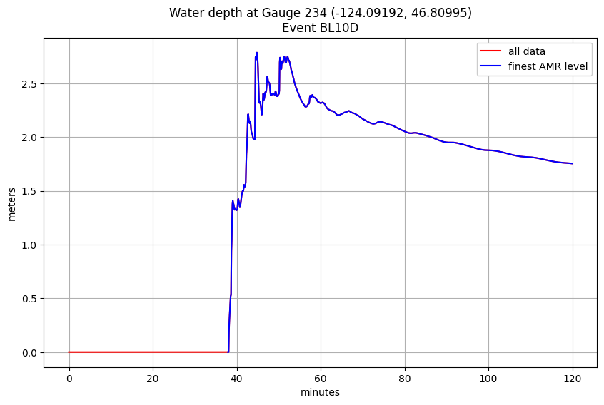

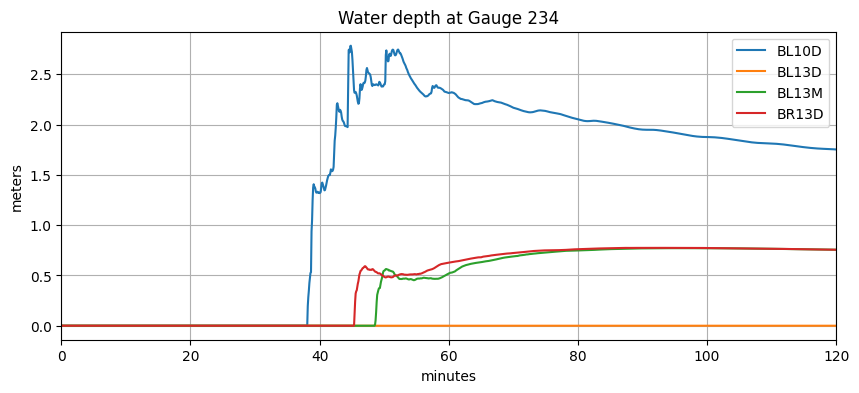
Plot all events at one gauge¶

Plotting h rather than hfine

all_events = ds.coords['event'].data  # all events
h_all = ds.h.sel(gaugeno=mygaugeno, event=all_events)

figure(figsize=(10,6))
for ev in all_events:
    plot(tminutes, h_all.sel(event=ev), label=ev)
legend()  # not very useful with 36 events
grid(True)
xlim(20,2*60)
xlabel('minutes')
ylabel('meters')
title('Water depth at Gauge %s' % mygaugeno);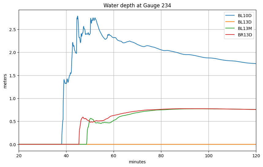

What’s the maximum value at this gauge over all events, and which event is largest?¶

From the plot above it’s hard to tell which event corresponds to the upper-most curve, so let’s look at the maximum depth at this gauge for each event:

print('The maximum depth over all time for all events is %.2f meters' % h_all.max())

The maximum depth over all time for all events is 2.78 meters

We can plot the maximum depth for each event separately:

hmax = h_all.max(dim='time')  # 1D array of 36 values for each event

figure(figsize=(6,3))
ievents = range(len(hmax.coords['event']))
plot(hmax.data, ievents)
yticks(ievents, hmax.coords['event'].data);
grid(True)
xlabel('meters')
title('Maximum water depth over 90 minutes at Gauge %i' % mygaugeno);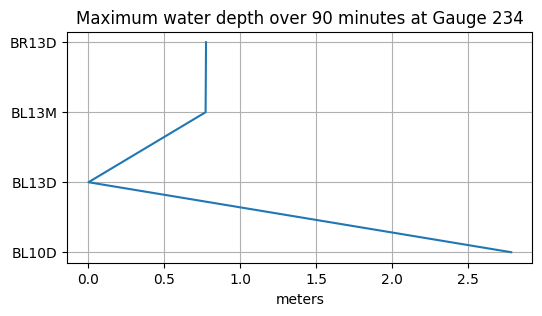

A more programatic way to determine which event has this maximum value is to use argmax:

imax = int(hmax.argmax(dim='event'))
emax = all_events[imax]
hmax = float(ds.h.sel(event=emax, gaugeno=mygaugeno).max())
print(f'Event {imax} named {emax} has the largest maximum depth at Gauge {mygaugeno} with value {hmax:.2f} m')

Event 0 named BL10D has the largest maximum depth at Gauge 234 with value 2.78 m

Plot this largest event to confirm:¶

figure(figsize=(10,6))
tminutes = gauge_t / 60.
plot(tminutes, h_all.sel(event=emax), 'b')
grid(True)
xlabel('minutes')
ylabel('meters')
title('Water depth at Gauge %i (%.5f, %.5f)\nEvent %s' % (mygaugeno,xg,yg,emax));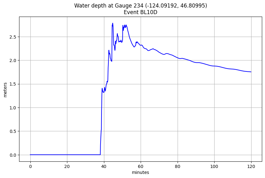

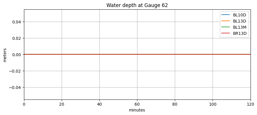
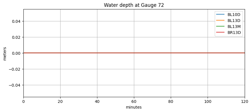
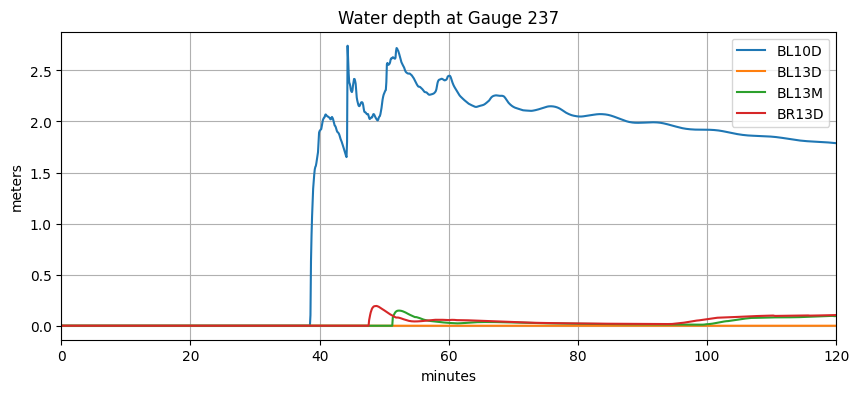
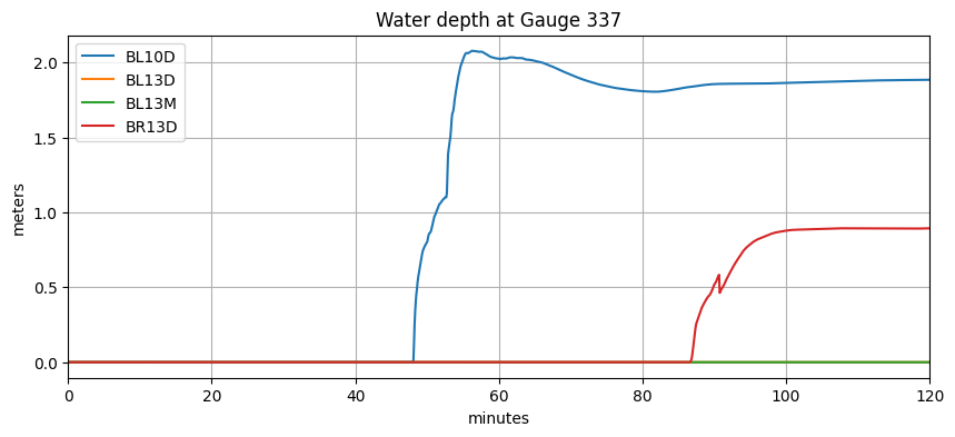
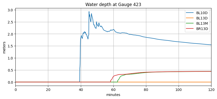
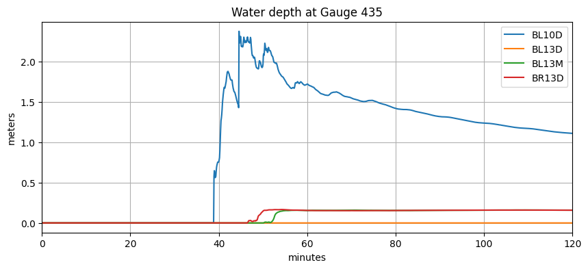
Plot all gauges for all events¶

For a small number of events and gauges, this is reasonable...

all_events = ds.coords['event'].data  # all events
all_gauges = ds.coords['gaugeno'].data

for gaugeno in all_gauges:
    h_all = ds.h.sel(gaugeno=gaugeno, event=all_events)
    
    figure(figsize=(10,4))
    for ev in all_events:
        plot(tminutes, h_all.sel(event=ev), label=ev)
    legend()  # not very useful with 36 events
    grid(True)
    xlim(0,2*60)
    xlabel('minutes')
    ylabel('meters')
    title('Water depth at Gauge %s' % gaugeno);