II.1: Overview of Numerical Simulations and Gepasi
In the second part of this guide, we will learn how to use numerical simulations to model enzyme behavior. Numerical simulations bear an advantage over analytical equations because they do not require the assumptions inherent in the traditional approach (covered in part I): the steady-state approximation, the free ligand approximation and the rapid equilibrium approximation. This means that numerical simulations can safely be used for complex kinetic schemes where the rate-determining step is not immediately apparent; for systems that involve multiple-tight binding interactions; and to simulate and fit data over a wider range of experimental conditions and time ranges than is possible with analytical equations.
Numerical simulations can provide both steady-state/equilibrium data and time-course data for all of the chemical species in a system. Starting from the same rate-law differential equations used to derive analytical equations, and the starting concentrations of the various species, numerical simulation programs increment the time by a small amount and calculate how the specific concentrations have changed. Time course data is generated simply by recording specific concentrations at each time point, while steady-state data are the specific concentrations at a time when the rates of change of the various species approach zero.
We will be using Gepasi (the General Pathway Simulator, freely available at www.gepasi.org) to demonstrate how numerical simulations are used. Unfortunately, Gepasi has a rather complicated and unintuitive user interface, but it is an extremely powerful simulation and fitting package. A word of warning: Gepasi is not the most stable piece of software, so save early and save often. Also, data generated by Gepasi are stored in several files in the same folder as your simulation (.gps) file. These data files are overwritten each time you run a simulation, so make sure you create a new folder (and copy the .gps file to it) for each new simulation.
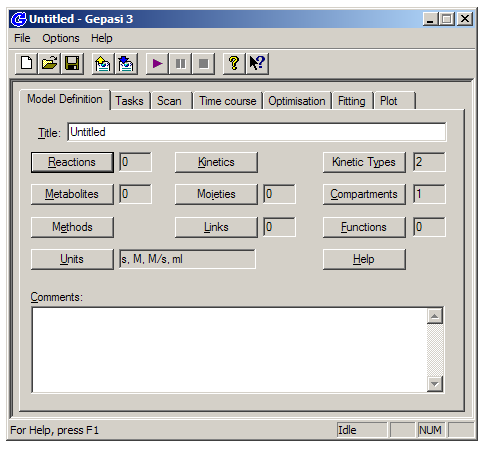
The interface is organized into seven tabs running across the top of the window. For any modeling task, you’ll want to proceed generally from left to right across the tabs. The first tab, ‘Model Definition’, allows you to specify all of the reactions in your system, as well as the associated rate constants and affinities. This tab also allows you to link the values of specific concentrations or rate constants to each other, and to define functions based on multiple specific concentrations.
The ‘Tasks’ tab allows you to choose between time-course and steady-state modes, while the ‘Scan’ tab allows you to simulate a range of different starting specific concentrations or rate constants. The ‘Fitting’ tab allows you to define fitting variables and perform a least-squares minimization to experimental data using a variety of fitting algorithm. Finally, the ‘Plot’ tab is where you can plot simulated time-course or steady-state data, or compared fitted simulations to experimental data.