|
|
|
Techniques for 3D Quantitative Echocardiography
LV Volume
Regional Wall Thickness
Regional LV Shape
Quantitative Mitral Annular Dynamics
LV Volume
LV volume is computed by summing the volumes of the tetrahedra formed by connecting a point inside the LV cavity with the vertices of each triangular face on the reconstructed 3D surface. The LV volumes determined at end diastole and end systole are used to calculate stroke volume, ejection fraction, and cardiac output, as well as the respective volume indices.
LV mass is calculated as the difference between the volumes of the LV endocardial and epicardial surface reconstructions, multiplied by the relative density of cardiac muscle. These measurements have been validated using in vitro hearts. 3D quantitation is more accurate than 2D because it avoids geometric assumptions.
Regional Wall Thickness
Standard 2D echocardiographic exams include qualitative assessment of regional and global left ventricular wall motion and thickening. From a few standard imaging planes, the systolic wall motion (movement of epicardial segments towards or away from the lumen)in each predefined sector is measured using calipers and assigned a semiquantitative score. Such visual assessments have limited sensitivity in differentiating between grades of abnormality and are poorly reproducible between observers. We sought to quantify regional ventricular function from the 3D surface reconstructions. Tomographic imaging modalities such as ultrasound depict epicardium as well as endocardium. Therefore, we focused attention on measuring regional wall thickening, since it is less subject to translational artifact than wall motion.
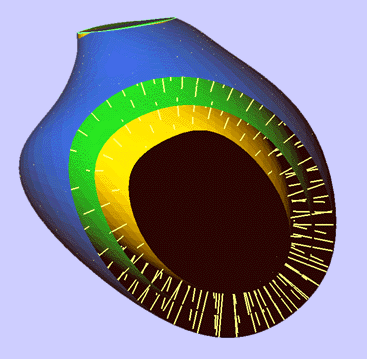
Regional wall thickness is measured using a 3D version of the Centerline LV angiographic wall motion method. A medial surface, called the CenterSurface™, is constructed midway between the epicardial and endocardial surface reconstructions. Chords are drawn perpendicular to the CenterSurface and extended to their intersection with the endocardium and epicardium. The length of each chord is a measure of the local wall thickness. Comparison of the wall thickness at end diastole and end systole at each triangular face of the LV surface provides a measure of wall thickening, a parameter of regional LV function. Below are a schematic and an application of the CenterSurface method.
 |
|
CenterSurface in action. Cutaway view
looking inside the endocardium and epicardium of the left ventricle; the CenterSurface is the green surface, and chords can be seen as short light yellow lines. |
 |
|
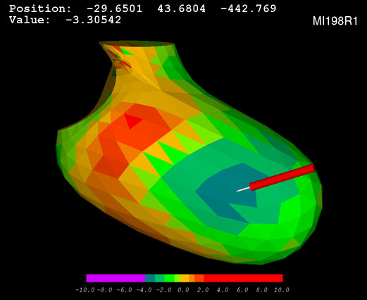
The CenterSurface method is applied to measure regional wall thickness at end diastole and end systole. Regional wall thickening is then computed as the change in wall thickness normalized by the end diastolic wall thickness. The analysis can be performed over the entire left ventricle.
The three dimensional display shows the location, extent, and severity of LV dysfunction. In this color scale, normal function is tan, hypokinesis is expressed by successively cooler shades, and hyperkinesis is indicated by warm colors. The stylus points to a region whose function is -3.3 standard deviations (below the normal mean).
|
Regional LV Shape
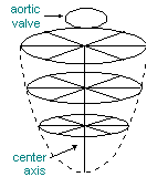
Regional LV shape is analyzed based on a center axis constructed from the centroid of the mitral valve to the furthest point on the epicardium (assumed to be the apex). A radial search is then performed to locate the position of points on the reconstructed LV.
To normalize for patient size, the distance from the center axis to the reconstructed surface is divided by center axis length. To standardize orientation, the centroid of the aorta at valve level is placed at 90 degrees (along the LV endocardial circle) and the angular coordinates of points on the LV are specified in a counterclockwise direction with the LV viewed from the apex.
The LV surface is then divided into 16 segments. Regional shape in each segment is calculated as the mean radial distance from the center axis of all points in that segment.
To see an example of regional shape analysis, click on the Schematic Center Axis diagram below.
 |
|
Regional shape analysis is based on the regional mean distance of LV segments from the center axis. This technique is useful for diagnosing, stratifying, and bioengineering modeling of a wide variety of cardiac diseases, including post-infarct remodeling, ventricular aneurysm, congenital malformations, and cardiomyopathy. |
Quantitative Mitral Annular Dynamics
Mitral annular size and shape parameters can be measured from the Fourier-derived reconstructions used to model them. Standard measurements are calculated as follows:
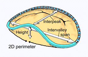
Mitral annulus orifice area is computed as the area projected onto the least-squares plane fitted to the annular curve. Area is indexed to body surface area.
3D perimeter length is defined as the path length along the fitted (nonplanar) annular curve; the 2D perimeter is the path length of of the least-squares plane projection of the 3D curve.
To calculate eccentricity, an ellipse approximating the annulus is constructed by matching its centroid and second moment of inertia to those of the area enclosed in the annular curve as projected onto the least-squares plane.
Annular height, interpeak span, and intervalley span are measured as shown below.
These measurements have been validated in phantoms in vitro. Although the analyses were developed initially for application to data acquired from rotational transesophageal echo scans, the measurements can also be made from transthoracic 3D echo scans6.
To learn more about quantitative mitral annular shape analysis, click on the mitral annulus diagram below.
 |
|
3D conceptualization of the mitral annulus as a nonplanar ring with local maxima anteriorly and posteriorly. Axes of measurement are shown. |
Back to Top
|