|
|
|
Division of Nuclear Medicine SimSETAppendix V: |
|
This document describes the implementation of Forced Detection Tables in the SimSET PHG module. It is intended to be background information for the programmer interested in understanding and/or modifying the PHG. It contains diagrams and descriptions of data structures used to manipulate Forced Detection data as well as algorithms for using the information they contain.
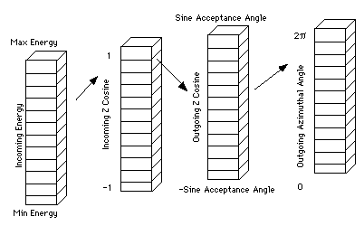
The Forced Detection tables contain pre-computed probabilities that a photon with a specific direction and angle will scatter in a selectable range of outgoing angles. In other words, the tables answer the question: For a given incoming direction and energy, what is the probability that the photon will scatter within a specific range? The specific range is computed to insure the photon will enter the detector within the acceptable angle.
In particular, the Forced Detection Tables convert from the coordinates used by the Klein-Nishina formula, incoming energy and scatter angle, to the coordinates needed to implement Forced Detection (incoming energy, outgoing z-direction cosine, and sine of outgoing azimuthal angle).
Using pre-computed tables eliminates the costly computation associated with the process.
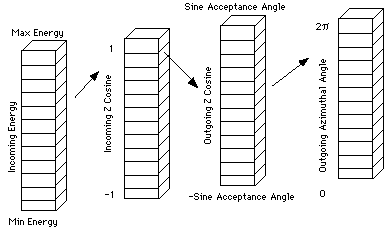
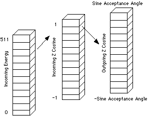
There are three Forced Detection Tables, each providing a different view of the Klein-Nishina distribution:


Once an interaction point has been selected along the line of travel through the critical zone a scatter angle must be chosen to insure detection. The algorithm for continuing is given below:
Compute the relative probability that the scatter angle will occur within the computed acceptable range. You must first calculate the "KNDensity table bin index" for the incoming energy, the incoming z cosine, the sine of the minimum acceptance angle and the sine of the maximum acceptance angle. These will be the same for all tables and are referred to as the incomingEnergyIndex, incomingZCosineIndex, minAcceptanceAngleIndex and maxAcceptanceAngleIndex.
probScatterInRange = KNDensCumTotal[incomingEnergyIndex]
[incomingZCosineIndex][maxAcceptanceAngleIndex] -
KNDensCum[incomingEnergyIndex][incomingZCosineBin]
[minAcceptanceAngleIndex ][0]
Pick a target probability from the acceptable range.
targetScatterProbability = KNDensCum[incoming energy]
[incomingZCosineBin][minAcceptanceAngleIndex ][0] +
(random number * probScatterInRange).
Now find the bin in the KNDensityCumulative Table that contains the selected targetScatterProbability.
This requires a search operation on the table. You know the incoming energy and incomingZCosineIndex; for those values you search through the table from outgoingZCosineIndex = minAcceptanceAngleIndex to maxAcceptanceAngleIndex, at each AzimuthalIndex, until you find an outgoingZCosineIndex and AzimuthalChangeIndex such that
KNDensCum[incomingEnergyIndex][incomingZCosineIndex]
[outgoingZCosineIndex][AzimuthalChangeIndex] < targetScatterProbability < KNDensCum[incomingEnergyIndex][incomingZCosineIndex]
[outgoingZCosineIndex][AzimuthalChangeIndex + 1]
or, if AzimuthalIndex + 1 is outside the range for azimuthal indices,
KNDensCum[incomingEnergyIndex][incomingZCosineIndex]
[outgoingZCosineIndex][AzimuthalChangeIndex] < targetScatterProbability < KNDensCumTotal[incomingEnergyIndex][incomingZCosineIndex]
[outgoingZCosineIndex]
This search gives us two values, the outgoingZCosineIndex and AzimuthalChangeIndex.
Select an outgoing z cosine.
The outgoingZCosineIndex computed above determines the range for the outgoing z cosine. The outgoing z cosine "zCosineOut" should equal the starting point of outgoingZCosineBin plus the size of outgoingZCosineIndex bin * a random number.
Select an outgoing azimuthal angle.
The AzimuthalChangeIndex computed above determines the range for the change in azimuthal angle. The outgoing azimuthal angle "azimuthOut" should equal the incoming azimuthal angle + (start of AzimuthalChangeIndex + range of AzimuthalChangeIndex* random number).
Determine xCosineOut and yCosineOut from azimuthOut
Compute the cosine of the scattering angle
CosScatteringAngle = (xCosIn * xCosOut) + (yCosIn * yCosOut) + (zCosIn * zCosOut)
Compute the outgoing energy
Compute the outgoing photon weight
WtOut = WtIn * ( KN( CosScatterAngle, incomingEnergy, outgoingEnergy ) / KNDensity[incomingEnergyIndex][incomingZCosineIndex]
[outgoingZCosineIndex][AzimuthalChangeIndex] )
where KN is the Klein-Nishina density function as given in equation 11 of Zerby (6).
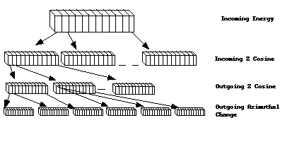
The diagrams above presented a logical view of the Forced Detection Tables. The diagram below re-iterates that view in a slightly modified fashion:

Because dynamically sized and allocated arrays are difficult to deal with in C, we chose to re-organize the data. From the discussion above, each photon arrives with an incoming energy and z direction cosine. Associated with these two variables are three relative probability values (outgoing z cosine, outgoing azimuthal change, cumulative outgoing azimuthal change). Using this information to form a new perspective on our data we have reorganized the data as diagrammed below:
Now we have a two-dimensional table where each element contains three arrays. The complexity of the data structure has been reduced at the expense of adding a complexity to our indexing. The organization maintains a reasonable relationship to the information.
Last revised by: Steven Vannoy Revision date: 12 Jan 1999