![[UW Pediatrics]](/bicg/images/uwp24.jpg)
SLIMMER
SLIMMER Manual
Kio Kim1, Piotr Habas1, Mads Fogtmann1, Vidya Rajagopalan1, Julia Scott1, Sharmishtaa Seshamani1, Francois Rousseau3, A. James Barkovich2, Orit Glenn2 and Colin Studholme11Biomedical Image Computing Group, Department of Pediatrics, Division of Neonatology, University of Washington, Seattle WA
http://depts.washington.edu/bicg
2Department of Radiology and Biomedical Imaging, University of California San Francisco, San Francisco, CA
3LSIIT, UMR 7005 University of Strasbourg, Illkirch, France
November 6, 2012
| RView Version: | 9.068 download |
| slimmerSIMC Version: | 1.18 |
| slimmerRecon Version: | 1.04 |
B. Loading
1. Open RView
2. Load SLIMMER tool
3. Select original DICOM directory
4. Select stacks to apply SLIMMER
C. Processing Data
1. Create Reference Image and Mask
(a) Select and orient reference stack
(b) Create reference mask
2. Stack Motion Estimation
(a) Scanner Align Non-Ref Stacks
(b) Auto Align Non-Ref Stacks
(c) Save All Stack Data
3. Slice Motion Estimation
4. Volume Reconstruction
D. Results
1. Final Inspection and Save
2. Motion Graph
3. Saved Files
References
*. Acknowledgement↑top
This software was created as a part of the NIH grant #NIH/NINDS R01 NS 055064. Users please cite the appropriate papers provided below when using this software in research publications.A. Introduction↑top
The Slice MRI Motion Estimation and Reconstruction (SLIMMER) tool is intended to allow the formation of a single 3D high resolution image from multiple sets of lower resolution multi-slice MRI data, where regional tissue motion can occur between the acquisition of slices. The input data is a set of raw DICOM format multi-slice data. The final output is a single volume image in GIPL or NIFTI format. The plugin tool for rview provides a graphical user interface to load data, automatically initialize the stack alignment from scanner coordinates, select the region of interest and then to inspect the result of regional between-slice motion estimation, bias inconsistency correction and volume reconstruction algorithms.The SLIMMER tool loads raw DICOM files, performs motion correction and builds a 3D reconstructed volume. SLIMMER tool forms stacks from raw DICOM images of 2D slice, and assists to align them to the reference space. It performs slice-stack and between-slice motion correction of user selected anatomical regions appearing in multiple multi-slice imaging studies and builds a full 3D volume from the motion scattered slice imaging data. It provides a graphic user interface to apply algorithms for the Slice Intersection Motion Correction (SIMC) [1][4], slice bias consistency correction [2][5] and 3D volume reconstruction [1][3].
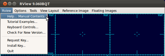
This manual focuses on how to use the SLIMMER tool to load data, how to apply stack and slice motion correction, and how to reconstruct the final 3D image. A general manual for RView can be accessed from the RView menu, by selecting RView-Help...Manual Contents. (You need an internet connection.)
B. Loading↑top
1. Open RView
Run RView by clicking the shortcut icon, or from the command line.Note: When running from the command line, use the full path and the binary name, i.e.,
| $ /full/path/to/binary/rviewqt |
2. Load SLIMMER tool
Select Tools-SLIMMER Motion Correction Tool to load SLIMMER tool.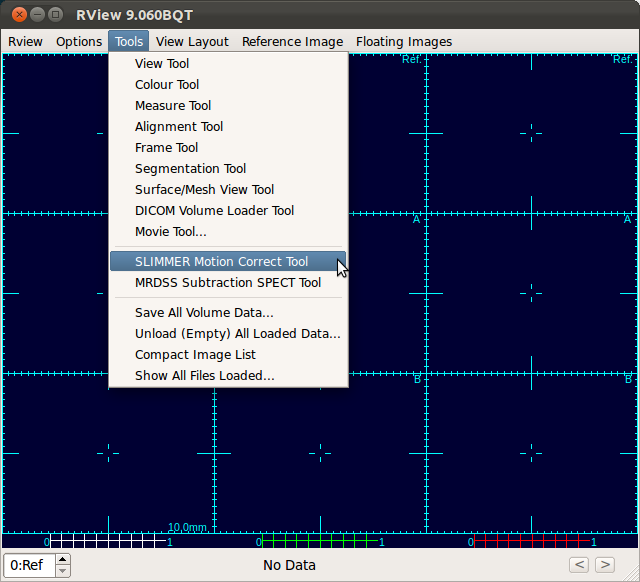
3. Select original DICOM directory
Selecting SLIMMER Motion Correction Tool from the menus will open a directory selection window. Navigate to the top directory that contains DICOM files to process and click Choose button to load all DICOM files within the subdirectories.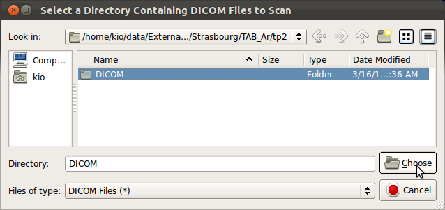
4. Select stacks to apply SLIMMER
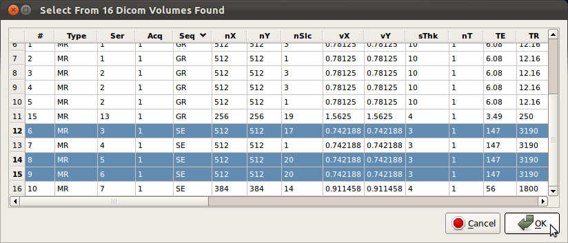
SLIMMER tool will parse all DICOM headers and display available images grouped by stacks. Seq column displays the sequence code for the stack acquisition, i.e., SE, GR, EP etc. SLIMMER tool is aimed at Fast Spin Echo sequences (SE) such as HASTE or SSFSE, so select only SE sequence stacks. You can find SE stacks by sorting the stacks by the sequence code by clicking Seq column label in the loading window. Check the numbers of slices (nSlc), voxel dimensions (vX, vY, sThk), TR and TE columns to ensure the values are comparable for consistent fusion of the data. Typical values for those variables are shown below.| Name | Abbrv. | Typical range |
| Number of slices | nSlc | >5 |
| In-plane voxel dimension | vX,vY | <1.5 mm |
| Slice thickness | sThk | <5 mm |
| Echo Time | TE | ~100 ms |
| Repetition Time | TR | >1500 ms |
Once you have selected stacks to load, click OK button to proceed.
Note: Some systems occasionally make duplicate copies of DICOM data as shown below. Use the horizontal scroll bar and check the acquisition time and date of the stacks to ensure that there exists only one copy at each acquisition time. If multiple copies with identical acquisition time are found, load and inspect them as they could be an original and a post-processed version of the original (for example, distortion or bias corrected version).
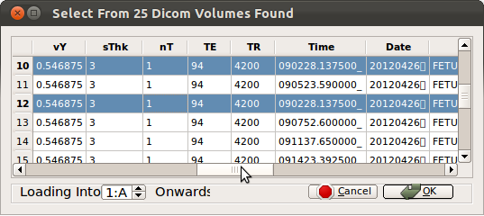
Once stacks are loaded, inspect them and remove undesired stacks as explained below. RView will automatically detect and warn if any stacks have identical acquisition time.
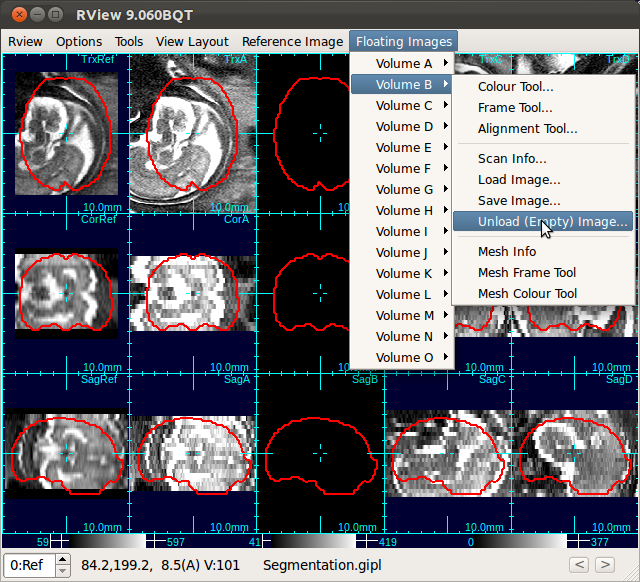
Note: If you want to exclude stacks from the process, you can unload stacks. For example, the stack B in the figure below (the third column) has a substantially different contrast from the rest of the stacks. In order to unload this stack, navigate to Floating Images→Volume B→Unload Image from the menu bar.
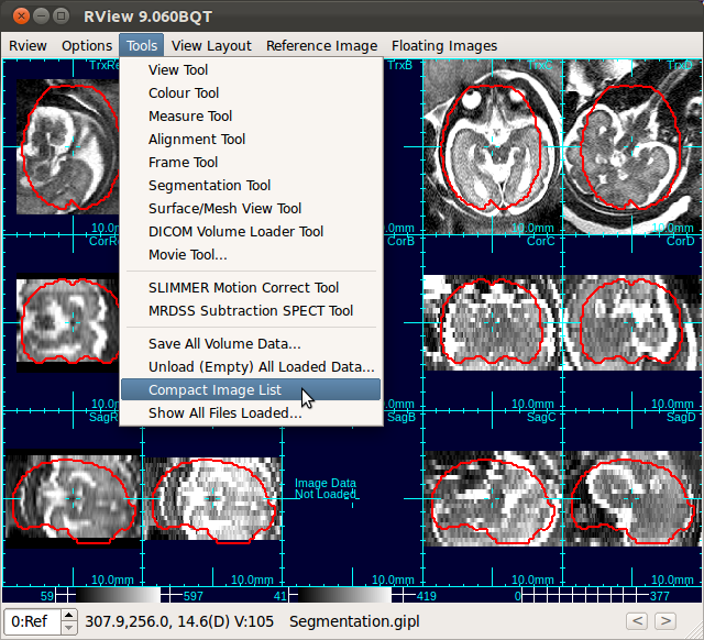
After unloading stacks, select Tools→Compact Image List to the remove blank columns.
C. Processing Data↑top
1. Create Reference Image and Mask↑top
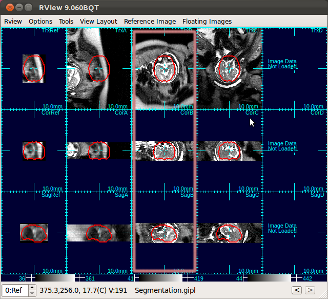
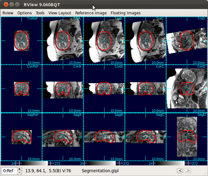
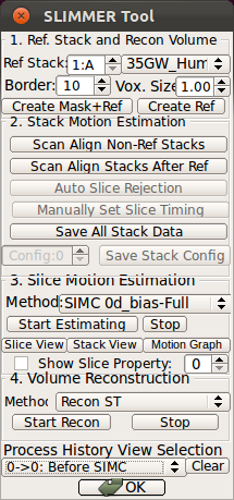
When RView finish loading stacks into viewer panels, the stacks will be displayed in the RView panels and SLIMMER tool window will pop up. The left most column is reserved for the reference image, although initially it will display arbitrary anatomy in the first stack. The rest of the columns will display the stack images, which are loaded in the order of the stack acquisition time.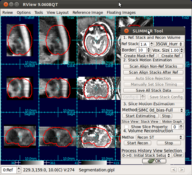
(a) Select and orient reference image
The first step of stack alignment is to generate a reference image from one of the stacks. A stack with the best quality, usually in axial orientation, is recommended for the reference stack. Input the stack index into Ref Stack box of the SLIMMER tool window. Use a numerical index instead of alphabet (A→1, B→2, etc.)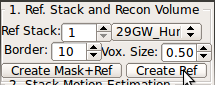
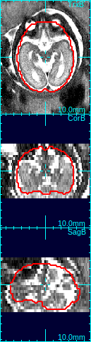
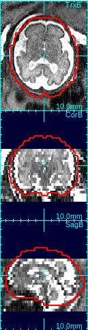
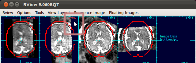
The figure below is an example screen of RView when SLIMMER finished loading DICOM files. In the top-right corner of each panel is a string indicating the view plane and the image name. The left-most column is the reference image (Ref), and is followed by columns of the stack images, alphabetically indexed. In this screen, the stack B (the third column) has all of the three view planes, namely, axial (Trx), coronal (Cor), and sagittal (Sag), correctly oriented, except that the head is upside down.
Input your choice in the Ref Stack box of the SLIMMER tool window.
In case you need to recenter or reorient the stack chosen for reference, open the alignment tool for that stack by selecting Floating Images→Volume Index→Alignment Tool...
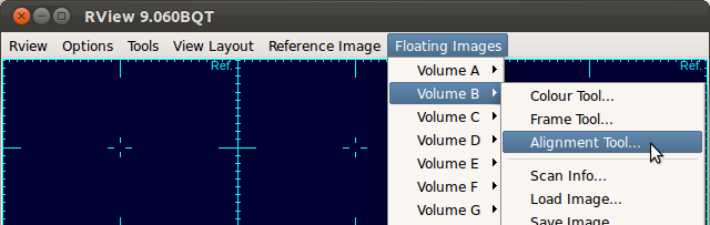
Center the stack (use O-key on the keyboard) and adjust the orientation (use Rotation slide bars in the alignment tool), so that the first, second and third view panels display axial, coronal and sagittal views of the brain, respectively. A detailed documentation on the alignment tool is included in RView help.
- O-key on the keyboard: Recenters the stack under the mouse cursor.
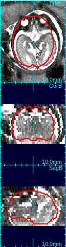
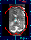
In the figure below, the first column shows that brain is off-centered, and upside-down. Move the mouse cursor to the center of the anatomy, and press o-key once (only once!), and the stack will be recentered so that the current cursor location will be the new center (second column in the figure below).
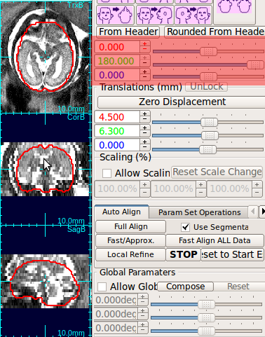
- Rotation slide bars: Adjusts the orientation of a stack.
Using the rotation slide bars, correct for the upside-down configuration---in this case, the image needs to be rotated by 180 degrees around the y-axis (the third column, pink box). Often times, the rotation might be complicated involving rotations around all axes. Use the rotation slide bars interactively to find the correct rotation angles.
 |
→ |  |
→ |  |
→ |  |
| Move cursor to the center of anatomy | Press o-key to recenter the stack | Use rotation slide bars to correct rotation | Recreate a mask with a correct size |
(b) Create reference mask
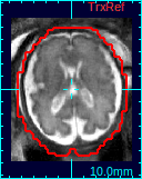
Select the best matching mask type using the mask type list in order to determine the size and shape of the reference mask. The options include the human fetal brains of various gestational age, the human adult brain, and the monkey brains. An ideal mask should include rigid tissues (brain and skull) as much as possible, and exclude maternal tissues and amniotic fluid. For example, the column 4 in the figure above demonstrates a good choice of mask size---it includes the whole brain and skull areas, and the maternal tissues/amniotic fluid regions are almost completely excluded from the mask area.Clicking Create Mask+Ref button will create a reference image from the selected original stack by interpolating it to the resolution specified in Vox. Size box. The contour of the age specific mask will be overlaid in view panels.
2. Stack Motion Estimation↑top
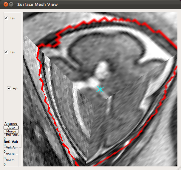
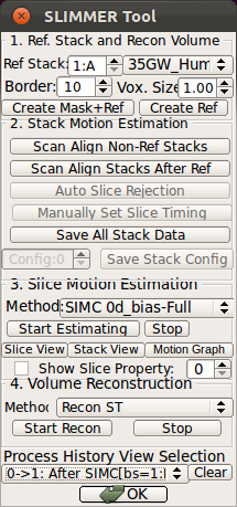
(a) Scan Align Non-Ref Stacks
Use Scan Align Non-Ref Stacks button to align non-reference stacks to the reference. This will bring the non-reference stacks to the same position as the reference stack.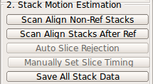
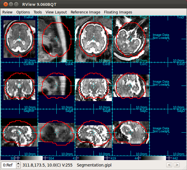 |
→ | 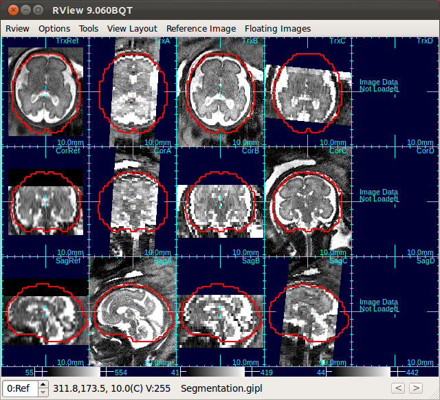 |
| Only Stack 2 is aligned | Click Scan Align Non-Ref Stacks |
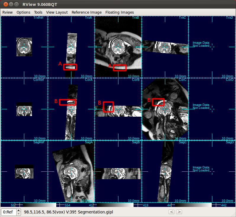 |
| A: Subcutaneous fat, B: bladder |
Scan Align Non-Ref Stacks automatically detects gimbal-locked stacks and corrects them.
(b) Scan Align Stacks After Ref
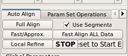
When the fetal motion between stack acquisitions is severe, use Scan Align Stacks After Ref button to progressively align stacks. When it is difficult to align all stacks to a single reference stack, Scan Align Stacks After Ref button is particularly useful.In order to compensate for the fetal motion between the reference stack and non-reference stacks, perform a stack-to-stack motion correction. RView provides an automated tool for a stack-to-stack alignment.
Use alignment tool for the non-ref stack before using the auto alignment to ensure that the non-ref is at least roughly aligned with the reference stack. (Read RView help on the use of the alignment tool.) Then, use Fast/Approx. alignment button. This will correct for gross motion of te fetal head in the non-ref image with respect to the head in the reference image.
If the auto alignment fails for any reason, click Reset to Start Estimate to revert the auto alignment. Repeat this for all non-ref stacks.
Before proceeding, check following items:
- Alignment: Use the alignment tool if there remains unresolved misalignment of stacks due to any abrupt motion between stack acquisitions or other reasons.
For example, in the below figure, the relative/ position of the fetus to the scanner have changed due to fetal and maternal motion, between the acquisitions of the stack C and the stack D (the fourth and fifth columns). In such a case, use the alignment tool to bring the stack D to the reference fetal brain coordinates.
- Gimbal lock: If a stack is gimbal-locked, click UnLock button in the alignment tool window to resolve it.
RView uses Euler angles to represent rotation. In this representation, rotation may suffer gimbal lock when the y-rotation becomes close to ±90 degrees. If this happens, Unlock button becomes activated. Click this button, and RView will rotate the stack to the gimbal unlocked position and modify Euler angles accordingly.
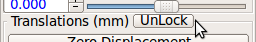
Make sure Unlock button is disabled for all stacks, before proceeding to the next step.
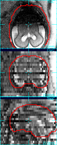
Note: Since Scanner Align Non-Ref Stacks button automatically detects gimbal-lock and unlocks it, use of Unlock button will be necessary only in limited circumstances. - Slice quality: If any slice is blurry, blank, or has any quality issue, move mouse cursor to the slice and press q-key on the keyboard. This will set the quality value of the slice to 0, and the slice will be colored in blue.
The low quality slices will be excluded from motion correction and volume reconstruction. For example, in the figure below, the axial slice is corrupted due to the fetal motion during the slice acquisition. Since the dark area does not reflect the actual anatomy, the image is not consistent with other intersecting images, and thus should be excluded from the motion correction step and the reconstruction step.
→ 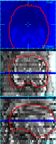
Move mouse cursor to a degraded slice. Press q-key to mark a low quality slice.
(c) Save All Stack Data
Once the dataset is stack-aligned, save the dataset by clicking Save All Stack Data button in Stack Motion Estimation box of SLIMMER tool window. This will open a directory selection window. Select the parent director of the DICOM directory, which will create SLIMMER directories in parallel with the DICOM directory. SLIMMER will generate a stack data directory for each stack (mrT2raw_n) and, and a SLIMMER workspace directory (mrT2raw_slimmer_R0).Below figure shows an example directory structure. User selected tp1, and SLIMMER directories were created in parallel with the DICOM directory.
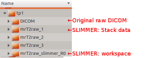
Each stack data directory includes following files:
| File name | Description |
| mrT2raw.gipl | Stack image data file |
| ref2mrT2raw.dof | Reference-to-Stack Rigid transformation file |
| ref2mrT2raw.sdof | Stack-to-Slice Rigid transformation file (motion uncorrected) |
| mrT2raw_scanTrans.dof | Scanner-to-Stack Rigid transformation file |
| mrT2raw_DICOMinfo.xml | |
| mrT2raw_GEOMinfo.xml | |
| mrT2raw_MRIinfo.xml |
The SLIMMER workspace directory includes following files:
Note: Drag-and-drop reconConfig.rvw into the RView window to reload the complete SLIMMER state.
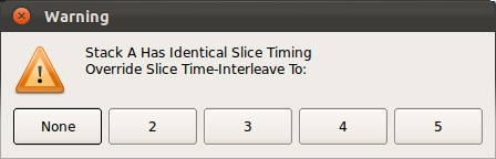
Note: When Save All Stack Data button is pressed, RView automatically check for the correctness of slice timing data of each stack, because the slice timing data provides correlation information between slice motion parameters. If a timing data corruption is detected, Manually Set Slice Timing button becomes activated. Then, user can click this button to manually reset the slice timing by choosing the actual interleaving factor.
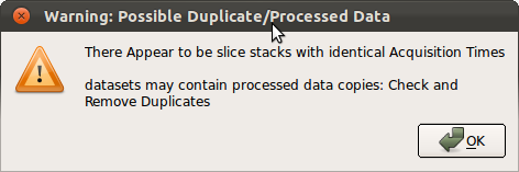
Note: When Save All Stack Data button is pressed, RView automatically checks if any loaded stacks have identical timing data. If identical timing data are detected, a warning window will pop up as below. Make sure to remove any redundant or before-processing stacks before proceeding.
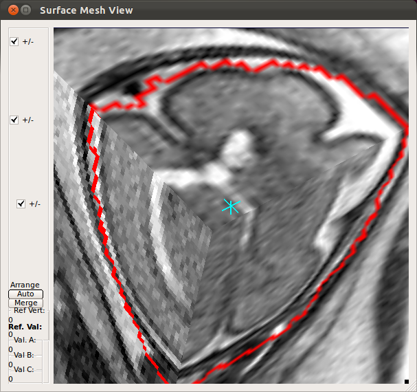
3. Slice Motion Estimation↑top
(1) Select motion correction method
When the dataset is in stack-aligned state, the slice motion estimation can be performed. This state can be also loaded to RView by drag-and-dropping a reconConfig.rvw file into an empty RView window.Select motion correction method in Slice Motion Estimation box-Method list.
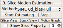
Slice motion is estimated by Slice Intersection Motion Correction [1] after bias stabilization [2]. User can select between two bias models for bias stabilization, and the slice motion scale for the motion correction. Available options are:
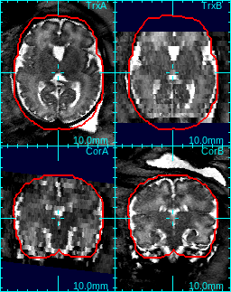
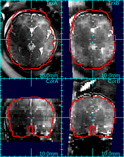
For example, in the figure below, the study in (a) has uniform 2D bias field, so 0th degree bias model is sufficient. On the other hand, the axial stack in (b) has a strong gradient in bias field when compared to the coronal stack, so 1st degree bias model is more suitable.
| (a) example of 0d bias | (b) example of 1d bias |
 |
 |
(2) Start Estimating
Clicking Start Estimating button will initiate a slice motion estimation process. This button will be disabled while the process is running, The running time varies from a few minutes to up to hours, depending on the number of image stacks, the amount of motion and the computation power. If the button becomes activated too soon (less than a few seconds), make sure you have installed RView correctly and try again.(3) SliceView and StackView
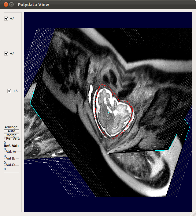
When the slice motion estimation is completed, use SliceView and StackView buttons along with Process History list to inspect the result. These buttons open a 3D viewer window, where you can rotate the view using the mouse. Use the mouse scrolling function (wheel) to zoom in and out.SliceView displays the slices in the 3D space with the current motion estimation. You can view different slices by clicking within the RView viewer panels, and SliceView will render slices at the cross-hair location.
- In order to turn on/off the visualization of a stack, move mouse cursor over to any panel of the stack, and use s-key on the keyboard.
This applies to the reference image as well. When the 3D visualization is off for a stack, the indicator string changes the color from cyan to red.
- Using Processing History list, alternate between the motion estimation before SIMC and after SIMC to make sure that the motion estimation was correctly done.
  |
→ |   |
StackView displays the location of entire slices of the stacks by drawing the edges of the slices. You can use s-key on the keyboard and Processing History list as explained for SliceView. This view is useful to see the motion of the subject within stacks. For example, StackView below shows two stacks, where the fetus has moved between the acquisition of individual slices. Slice edge color is white by default, but if Show Slice Property checkbox is checked, it colors the slice edges according to the slice mismatch energy as defined in .smatch file.
  |
→ | 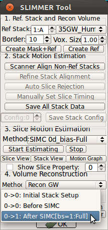  |
Note: Each line of Processing History list has the format of '(previous state)->(current state):(description of current state)'.
For example,
|
0->1:After SIMC[bs=1:Full] |
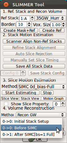
4. Volume reconstruction↑top
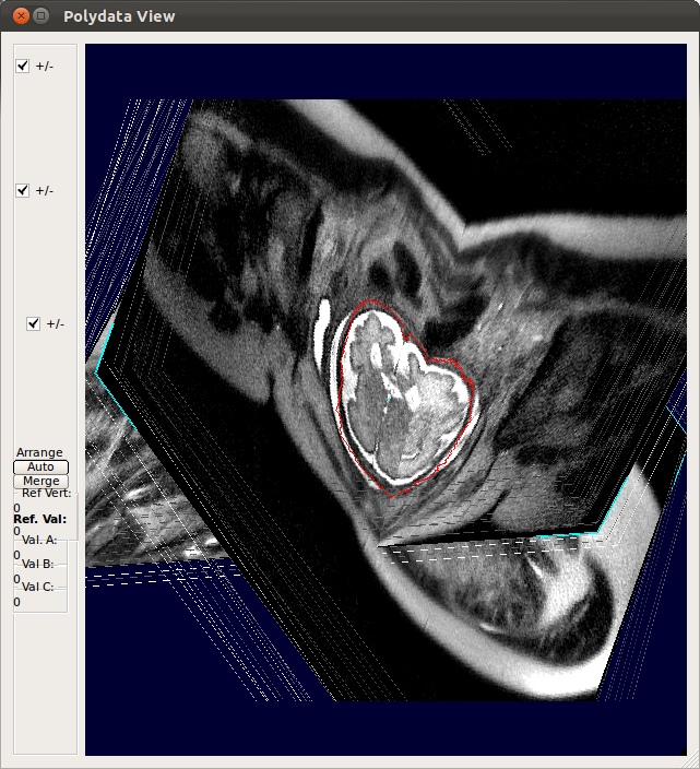
(1) Select volume reconstruction method
Currently two reconstruction methods are available: Gradient weighted Gaussian averaging (GW)[2] and Structure tensor averaging of neighbors (ST)[3].
(2) Start Recon
Clicking Start Recon button will initiate a reconstruction process. This button will be disabled until the reconstruction process is completed. If the button becomes activated too soon (less than a few seconds), make sure you have installed RView correctly and try again.(3) Process History list
If a 3D volume is reconstructed, a new state will be added to Process History list. Select the new reconstruction state, and the reconstructed volume will appear in the reference panel of RView.You can compare the results with the initial reference volume, or other reconstructions using the Process History list.
 |
 |
 |
| Original ref. | GW recon. | ST recon. |
D. Results↑top
1. Final Inspection and Save↑top
After loading the reconstructed volume to the reference window using Process History list, inspect the reconstructed volume. In order to take a closer look, use F1-key to switch to a single stack image volume view of the reference volume.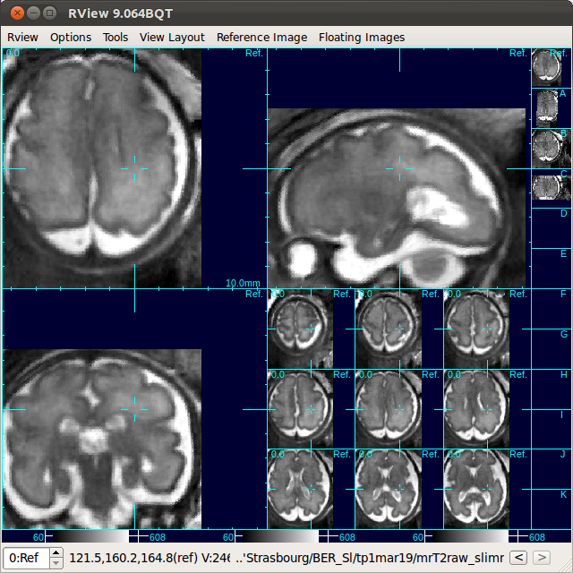
(In order to return to SLIMMER view, select Tools-SLIMMER Motion Correction tool again.) Although the reconstructed volume is saved in the SLIMMER workspace, user can resave the reconstructed volume in a different format/location by selecting Reference Image-Save Image... in the menu bar. In order to save the image in GIPL format, add .gipl as the file extension, or add .nii for NIFTI format.
2. Motion Graph↑top
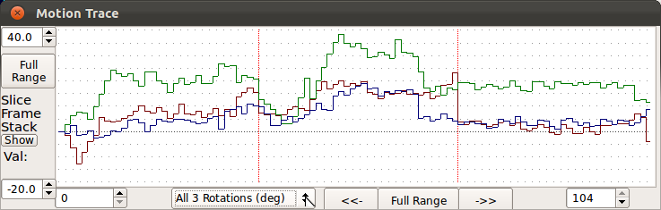
Use Motion Graph button to plot the estimated rotation and translation parameters as a function of the slice acquisition time, relative to the original planned location within the scanner. The plot is ordered on the time of slice acquisition and divided into sections (red bars) for each slice stack. Regions in blue on the trace indicate low quality slices (What is a slice quality?).The trace is updated as the user selects different processing stages (eg. before SIMC/after SIMC).
Note: No plot will be produced if the DICOM data did not contain valid slice timing information.
3. Saved Files↑top
In stack data directories, SLIMMER tool will generate slice motion parameters file (ref2mrT2raw_1.gipl) and slice bias consistency correction parameters file (ref2mrT2raw_1.sibc), and copies of them that might have been used for volume reconstruction.Each SLIMMER operation such as motion correction or volume reconstruction creates a new RView state, and each state is stored in the RView config file (reconConfig_n.rvw, where n is the sequence index number.) Each SLIMMER operation that involves a new slice motion estimation creates a new recon config file (reconConfig_m.txt), where m is the recon config index number (is different from the sequence index number!). All SLIMMER transactions will be logged in reconConfig.seq file. When a volume reconstruction was performed, the reconstructed 3D image is saved in mrT2raw_n.gipl, where n is the sequence index number, and replaces the reference image that was generated at the beginning of SLIMMER process.
| File name | Description |
| mrT2raw_n.gipl | 3D reconstructed image |
| reconConfig.seq | Sequence file of the process history |
| reconConfig_n.rvw | RView configuration file for each step in the process history |
| reconConfig_n.txt | Process configuration file for each step in the process history |
| reconConfig_n.log | Process log file for each step in the process history |
References↑top
[1] K. Kim, P. A. Habas, F. Rousseau, O. A. Glenn, A. J. Barkovich, and C. Studholme, "Intersection based motion correction of multislice MRI for 3-D in utero fetal brain image formation," IEEE Trans. Med. Imaging, vol. 29, no. 1, pp. 146-158, January 2010 .[2] K. Kim, P. A. Habas, V. Rajagopalan, J. A. Scott, J. M. Corbett-Detig, F. Rousseau , A. J. Barkovich, O A. Glenn, and C. Studholme, "Bias field inconsistency correction of motion-scattered multislice MRI for improved 3D image reconstruction," IEEE Trans. Med. Imaging, vol. 30, no. 9, pp. 1704-1712, September 2011.
[3] K. Kim, P. A. Habas, V. Rajagopalan, J. A. Scott, F. Rousseau , A. J. Barkovich, O A. Glenn, and C. Studholme, "Robust 3D reconstruction from motion scattered multislice MRI using second order models and structure tensor weighted kernel regression," MICCAI Workshop: Image Analysis of Human Brain Development, pp. 104-111,September, 2011.
[4] K. Kim, M. F. Hansen, P. A. Habas, F. Rousseau, O. A. Glenn, A. J. Barkovich, and C. Studholme, "Intersection-based registration of slice stacks to form 3D images of the human fetal brain," in Proc. IEEE International Symposium on Biomedical Imaging: From Nano to Macro, pp. 1167-1170, May 2008.
[5] K. Kim, P. A. Habas, V. Rajagopalan, J. A. Scott, J. M. Corbett-Detig, F. Rousseau, O. A. Glenn, A. J. Barkovich, and C. Studholme, "Non-iterative relative bias correction for 3D reconstruction of in utero fetal brain MR imaging," in Proc. 32nd Annual International Conference of the IEEE Engineering in Medicine and Biology Society, September 2010.
< END >
© 2024 Biomedical Image Computing Group, Division of Neonatology
Department of Pediatrics, University of Washington. All rights reserved.
Privacy |
Terms | Contact Us