«Tutorial Main   ‹prev  next› 

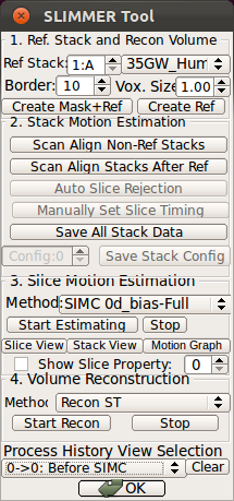
D. Slice motion estimation

When the dataset is in stack-aligned state, the slice motion estimation can be performed. This state can be also loaded to RView by drag-and-dropping a reconConfig.rvw file into an empty RView window.
Select motion correction method in Slice Motion Estimation box-Method list, and then click Start Estimating button to initiate a slice motion estimation process.

1. Motion estimation methods

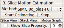
Slice motion is estimated by Slice Intersection Motion Correction [1] after bias stabilization [2]. User can select between two bias models for bias stabilization, and the slice motion scale for the motion correction. Available options are:

SIMC 0d bias-Full: 0th degree polynomial bias model, full scale motion correction

SIMC 1d bias-Full: 1st degree polynomial bias model, full scale motion correction

SIMC 0d bias-Refine: 0th degree polynomial bias model, motion correction refinement only

SIMC 1d bias-Refine: 1st degree polynomial bias model, motion correction refinement only

A typical study can be processed with SIMC 0d bias-Full. If the images have strong within-slice bias inhomogeneity, 1st degree model is useful.
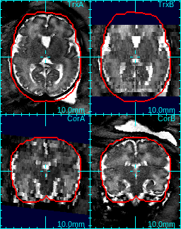
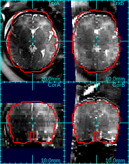
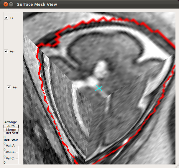
For example, in the figure below, the study in (a) has uniform 2D bias field, so 0th degree bias model is sufficient. On the other hand, the axial stack in (b) has a strong gradient in bias field when compared to the coronal stack, so 1st degree bias model is more suitable.

(a) example of 0d bias	(b) example of 1d bias

Use SIMC (0 or 1)d bias-Refine if a refinement is needed to currently motion corrected dataset.

2. Running time for motion estimation

The running time varies from a few minutes to up to hours, depending on the number of image stacks, the amount of motion and the computation power. Below are a few records from actual runs on a linux machine with Intel Core i7 (Quad Core with hyperthreading) 2.0GHz CPU,

7 stacks (2 axial, 3 sagittal, 2 coronal) 182 slices: 13 minutes

5 stacks (2 axial, 2 sagittal, 1 coronal) 129 slices: 5 minutes

3 stacks (1 axial, 1 sagittal, 1 coronal) 69 slices: 8 minutes

9 stacks (3 axial, 3 sagittal, 3 coronal) 325 slices: 117 minutes

Clicking Start Estimating button will initiate a slice motion estimation process. This button will be disabled while the process is running. If the button becomes activated too soon (less than a few seconds), make sure you have installed RView correctly and try again.

3. Checking the result

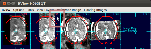
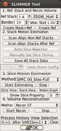
When the slice motion estimation is completed, you can use SliceView and StackView buttons along with Process History list to inspect the result. These buttons open a 3D viewer window, where you can rotate the view using the mouse. Use the mouse scrolling function (wheel) to zoom in and out.

(1) Slice View

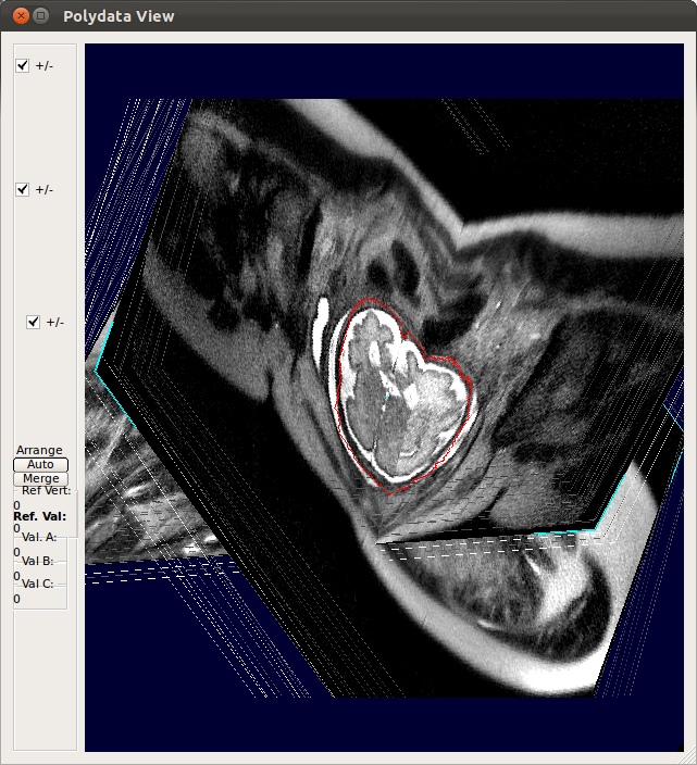
SliceView displays the slices in the 3D space with the current motion estimation. You can view different slices by clicking within the RView viewer panels, and SliceView will render slices at the cross-hair location.

• In order to turn on/off the visualization of a stack, move mouse cursor over to any panel of the stack, and use s-key on the keyboard. This applies to the reference image as well. When the 3D visualization is off for a stack, the indicator string changes the color from cyan to red.
  
  
• Using Processing History list, alternate between the motion estimation before SIMC and after SIMC to make sure that the motion estimation was correctly done.

→

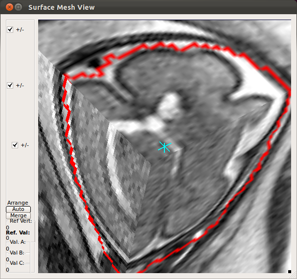(2) Stack View

StackView displays the location of entire slices of the stacks by drawing the edges of the slices. You can use s-key on the keyboard and Processing History list as explained for SliceView. This view is useful to see the motion of the subject within stacks. For example, StackView below shows two stacks, where the fetus has moved between the acquisition of individual slices. Slice edge color is white by default, but if Show Slice Property checkbox is checked, it colors the slice edges according to the slice mismatch energy as defined in .smatch file.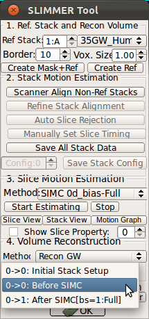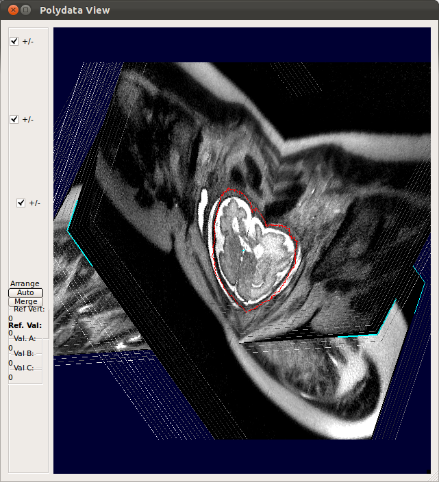

→

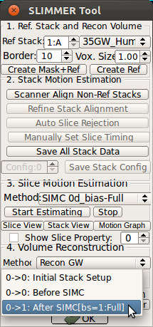Note: Each line of Processing History list has the format of '(previous state)->(current state):(description of current state)'.
For example,

0->1:After SIMC[bs=1:Full]

describes that the current state 1 is achieved from state 0 by treating the full SIMC with 1st degree bias stabilization.

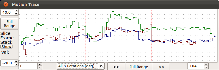
(3) Motion Graph

Use Motion Graph button to plot the estimated rotation and translation parameters as a function of the slice acquisition time, relative to the original planned location within the scanner. The plot is ordered on the time of slice acquisition and divided into sections (red bars) for each slice stack. Regions in blue on the trace indicate low quality slices (What is a slice quality?).
The trace is updated as the user selects different processing stages (eg. before SIMC/after SIMC).
Note: No plot will be produced if the DICOM data did not contain valid slice timing information.






«Tutorial Main   ‹prev  next›