|
 |
|
|
Overview
The Binning Module is used to process photon and detection records. It can be used during the simulation as each record is accepted (on-the-fly), or it can be used after the simulation via processing a standard history file. We call it the binning module because it "bins" data into multi-dimensional histograms. For example, the common "sinogram" is a two dimensional histogram where photon or detection records are binned according to their transaxial distance and azimuthal angle. The binning module will create histograms based on several different parameters which are described below.
Features
There are a number of features which help the user accumulate and process data with the binning module.
- User Specified Ranges: For most parameters the user may specify a minimum and maximum acceptable value. All photons that fall within this range are included in the histogram while the others are discarded.
- Summing Sequential Simulations: Although individual simulations can not be intermittently stopped and restarted, the results of sequential simulations can be summed together. The binning module uses information from the histogram header to scale the results appropriately.
- Specifying Output Format: The user can determine the resolution of the histograms. For integer data one, two, and four byte integers may be specified. For floating point data four and eight byte precision may be specified.
- Control Over Run-Time Precision: The user may wish to have single precision data files but need double precision summing while the histograms are being created. When doing multi-dimensional and/or large-range binning the memory requirements can easily become excessive. If double precision summing is not necessary single precision can be used.
- Ordering Histogram Dimensions: For two or more dimensions the ordering of the data must be considered. Previous versions of the PHG enforced a fixed ordering. With version 2.5 the order of the data corresponds to the order specified in the parameter file. For example if the first parameter listed is azimuthal angle and the second parameter is transaxial distance. Then the most quickly varying parameter (columns) will be transaxial distance and the most slowly varying parameter (rows) will be azimuthal angle.
- Counts, Weights, Weights Squared: The purpose of the PHG is to generate and propagate photons according to the object specifications and to characterize the escaping photons according to a number of criteria, such as position, direction, and energy. One statistic that can be binned is the simple count of photons. However, the PHG will never simulate the actual number of decays naturally produced in a real scan, it will always simulate a smaller number of decays. Consequently, each decay is assigned a weight which is determined by the volume in which it is generated, the amount of isotope assigned to that volume and the number of decays being simulated. Hence the weight is a number which can be used to easily convert histogram values to expected real-scan count rates. Furthermore, importance-sampling methods must weight photons to compensate for preferentially sampling "more productive" photons over "less productive" photons. When using these techniques, the count data are biased, whereas the correctly weighted data (the "weights" output by SimSET) provide unbiased estimates of the flux being considered. Finally, to correctly estimate the variance of the histogrammed weights, the weights-squared for each event are also histogrammed. For more information working with weights, see the section Estimating mean, variance, and number of counts from SimSET data below. Please see footnote 5 (Haynor et al 1991) for a detailed discussion of variance estimation with importance sampling.
- Multiple Binning Parameter Files: WE ARE FINDING SOME PROBLEMS WITH THIS FEATURE--IT DOES NOT ALWAYS WORK, IN SOME CASES THE BINNED DATA IS ZEROED OUT. HOWEVER, THE USER CAN STILL CREATE MULTIPLE BINNING FILES USING THE NEWLY ADDED TOMOGRAPH FILE FEATURE. In order to analyze different aspects of a single simulation on-the-fly, the user may specify more than one binning parameter file in the run-time parameters. The current limit on the number of simultaneous parameter files is twelve. This number can be increased by modifying the constant, PHG_MAX_PARAM_FILES, defined in the file PhgParams.h. The user must specify unique names for all histogram files in this case, failure to do so will prevent the simulation from executing.
- History Files: The binning module supports the creation of a history file which contains only the photons and detection records which have been accepted by the binning module. To use this feature you must specify the parameters "history_file" and "history_params_file" in the binning parameters file. See history files for more information.
Run-time screen output
When executing the simulation the binning module, several run-time statistics, such as the number of blue/pink photons (see the history file page) which reach the module, the number accepted by the module, and some weight statistics related to the accepted photons are reported on-screen. This can be helpful diagnostic information and should be noted.
Histogram file format
There are two parts to a histogram file (also known as an 'image file'), the header and the data. The header is a binary component with size equal to 32768 bytes. The header is explained in detail in the Header page. Basically all of the parameters that are used to specify the simulation are retained in the header as well as a few run-time statistics. There are utilities available for displaying the header (displayheader, printheader, print.header.c).
The format of the data portion of the histograms is largely controlled by the parameters as described in the section on configuration. It is essentially "raw" data. For example, if you specified to bin ten transaxial distance bins in single-precision real format then the size of your file would be 32768 + (10 * sizeof(float)), which is 32768 + 40.
convert is a useful utility for extracting data from histogram files - amongst other things, it can convert raw data to ascii text for use in spreadsheets.
Activating the Binning Module
To activate the binning module, edit the PHG run-time parameters file and enter a file name in the 'bin_params_file' field. Then create (or modify) a binning parameters file as described below.
Note: you can bin the data in up to 12 different ways simultaneously in any one simulation run. Just specify up to 12 unique binning parameter files in the PHG run-time parameters file.
As with the other SimSET modules, the binning module uses a parameter file to select binning and processing options, and to select histogram output files. The binning module parameters file is an ascii text file consisting of entries of the following format:
DATA_TYPE parameter_name = value For example,
BOOL do_ssrb = TRUE Type definitions for the relevant parameters are specified below.
[top of page] [example binning parameter files]
Parameter ordering
The order in which the bin parameters are specified in the parameters file is very important. The data will be ordered in the histograms according to the ordering of the dimensions in this file, going from slowest varying to fastest varying, top to bottom. Hence the first dimension specified in this file will vary the slowest while the last dimension specified in this file will vary the fastest.
Setting binning ranges
Setting the number of bins for any 'num_?_bins' type parameter to zero will cause the binning module to ignore that parameter entirely - events will be binned into a single bin according to the limits set in the other modules. Setting the number of bins equal to one will cause the binning module to filter photon/coincidence values according to the minimum and maximum you specify in the binning module - thus, if you have a z-range of +/- 10 cm in your detector module, but a z range of +/- 5cm in the binning module, a single bin containing only those events falling within the z range of +/- 5 cm will be created. Setting the number of bins greater than one will cause the binning module to bin into the specified number of bins within the specified limits.
[top of page] [example binning parameter files]
Binning according to event properties
Binning according to photon energy:
Set num_e_bins to the number of energy bins, min_e to the minimum acceptable energy, and max_e to the maximum acceptable energy (in keV): photons outside this range (and any coincidences involving them) are discarded.
For PET, the energy bins are two dimensional, one index for each photon, i.e.,
INT num_e_bins = 2
REAL min_e = 350.0
REAL max_e = 650.0would results in a 2x2 array of energy bins,
Photon 1 energy between 350 and 500 Photon 1 energy between 500 and 650 Photon 2 energy between 350 and 500 Photon 2 energy between 500 and 650 (Note that as there is no difference between Photons 1 and 2, the upper right and lower left bins can be summed together without any loss of information. SimSET does keep them separate, however.)
Binning according to scattering/randoms history:
SimSET can separate events according to whether they are primary, scatter, or, for PET, random events. The user chooses whether to accept random events (for PET), the minimum and maximum number of scatters to accept, and how to histogram the primaries, scatter and randoms. In determining the number of scatters, only scatters in the object and collimator are counted. Photons with the number of scatters outside the given range are discarded, as are coincidences involving them. (Note that there is no way of ignoring the range, if you don't want to restrict the number of scatters set the maximum value to a large number like 100). These parameters are assigned as follows:
BOOL accept_randoms = true
INT scatter_random_param = 6
INT min_s = 0
INT max_s = 100For PET the user accepts or rejects random events using the 'accept_randoms' parameter. The parameters min_s and max_s give the minimum and maximum number of photon scatters to accept. The parameter 'scatter_random_param' controls how the various types of events (primary, scatter, random) are histogrammed and how many indices are used:
scatter_random_param = 0 to combine primaries, scatters, and randoms
scatter_random_param = 1 to have a single index with two bins, one for all the non-scattered events (for PET this will include randoms where neither photon has scattered, if accept_randoms is true) and one with all events with one or more scatters (a PET coincidence is binned as scatter if either photon has scattered)
scatter_random_param = 2 to bin by number of scatters into (max_s-min_s)+1 bins for SPECT, ((max_s-min_s)+1)*((max_s-min_s)+1) bins for PET (each photon has a separate index). Photons with scatter counts below min_s or above max_s are discarded.
scatter_random_param = 3 is the same as scatter_random_param = 2 except that photons with scatter counts >= max_s are histogrammed into the maximum index value rather than discarded.
scatter_random_param = 4 (PET-only) to histogram coincidences into one index with (max_s-min_s)+1 bins using (blueScatters + pinkScatters) to compute the index number. The coincidence is rejected if the sum is < min_s or > max_s.
scatter_random_param = 5 (PET-only) is the same as scatter_random_param = 4 except that coincidences with (blueScatters + pinkScatters)>= max_s are histogrammed into the top index rather than discarded.
scatter_random_param from 6-10 are the same as 1-5 except that randoms are histogramed separately into an extra bin. The randoms bin is always the last bin. For options where the two photons are each given their own index (i.e., scatter_random_param = 6 or 7), the two photon indices are combined into a single linear index with one extra bin at the end for the randoms.
scatter_random_param = 6 (PET-only) to have three bins: one for true unscattered coincidences, the second for non-random scattered coincidences, the third for random coincidences.
scatter_random_param = 7 (PET-only) to have the same binning as scatter_random_param = 2 except with an extra bin for randoms, i.e., non-random coincidences are binned as with 2, but all random coincidences are binned separately to an extra bin at the end of the array.
scatter_random_param = 8, (PET-only) to have the same binning as scatter_random_param = 3 except with an extra bin for randoms, i.e., non-random coincidences are binned as with 3, but all random coincidences are binned separately to an extra bin at the end of the array.
scatter_random_param = 9,(PET-only) to have the same binning as scatter_random_param = 4 except with an extra bin for randoms, i.e., non-random coincidences are binned as with 4, but all random coincidences are binned separately to an extra bin at the end of the array.
scatter_random_param = 10, (PET-only) to have the same binning as scatter_random_param = 5 except with an extra bin for randoms, i.e., non-random coincidences are binned as with 5, but all random coincidences are binned separately to an extra bin at the end of the array.
[top of page] [example binning parameter files]
Binning into different histogram formats
Note: formats other than sinograms or 3D-RP projections may be obtained by varying the order in which the binning parameters are specified in the parameter file. See Parameter Ordering above.
Creating sinograms:
Set 'num_z_bins' to the required number of axial slices (this might correspond to the number of detector rings in a PET tomograph).
Set 'min_z' = the smallest value of z for binning.
Set 'max_z = the largest value of z for binning.
Note that these should be set to the minimum and maximum edges of the outer slices, respectively, not to the mean value of the slices. Any photon detected at a z position less than min_z or greater than max_z will be discarded.Set 'num_aa_bins' = the number of azimuthal angle bins. For SPECT, if this value is greater than 1, then it must be the same as the number of collimator positions. For SPECT, the range for the azimuthal angle runs from -180 to 180 degrees. For PET, the azimuthal angle runs from -90 to 90 degrees.
Set 'num_td_bins' = the required number of transaxial distance bins (i.e. the number of elements in a 1-D projection).
Set 'min_td' = the smallest value of transaxial distance for binning.
Set 'max_td' = the largest value of transaxial distance for binning.For SPECT, the data will be histogrammed by transaxial distance, azimuthal angle and z.
For PET, the data will be histogrammed by transaxial distance, azimuthal angle, z1 and z2 (the detected z position of the two coincident photons). These indices support PVI (3D PET), though one can also choose 3D-RP binning. To simulate 2D PET, you will need to extract the required 2D dataset from the 3D output, either by looking only at direct slices or by using single- or multi-slice rebinning.
For PET, sinogram data may be pre-processed for single-slice rebinning (Daube-Witherspoon and Muehllehner 1987) or for multi-slice rebinning (Lewitt et al 1994) by setting the variables 'do_ssrb' or 'do_msrb' TRUE or FALSE.
If MSRB is set TRUE, then set the 'detector_radius' variable to the appropriate detector radius. This is also needed for accurate binning with SSRB when using DHCI.
[top of page] [example binning parameter files]
Creating projections for 3D-RP:
3D-RP binning is currently only supported for PET simulations.
The spatial coordinates for the 3D reprojection algorithm (Kinahan and Rogers, 1990) are as follows:
z is parallel to the tomograph axis;
x is the horizontal axis perpendicular to z;
y is the vertical axis perpendicular to x and z.The projection coordinates xr, yr, theta and phi for 3D-RP are defined as follows:
Given a vector k normal to a particular projection plane and pointing away from the origin,
phi is the angle that the projection of k on the x-y plane makes with the y-axis;
theta is the angle that the projection of k on the x-y plane makes with itself;xr and yr are mutually perpendicular;
theta = 0 implies that yr = z; and
xr.z = 0.Set 'num_theta_bins' to the number of theta projection angles.
Set 'max_theta' to the largest theta angle for which there will be a projection. (min_theta is automatically set to -max_theta.)
Set 'num_phi_bins' to the number of phi projection angles. phi will range from 0 to 180 degrees for PET.Set 'num_xr_bins' = the number of bins along a projection in the xr direction.
Set 'min_xr' = the start point of the projection in the xr direction.
Set 'max_xr' = the end point of the projection in the xr direction.Set 'num_yr_bins' = the number of bins along a projection in the yr direction.
Set 'min_yr' = the start point of the projection in the yr direction.
Set 'max_yr' = the end point of the projection in the yr direction.
[top of page] [example binning parameter files]
Binning by crystal pair:
When block detectors are used SimSET can bin by crystal pair (or, for SPECT or singles binning of PET data, by crystal).
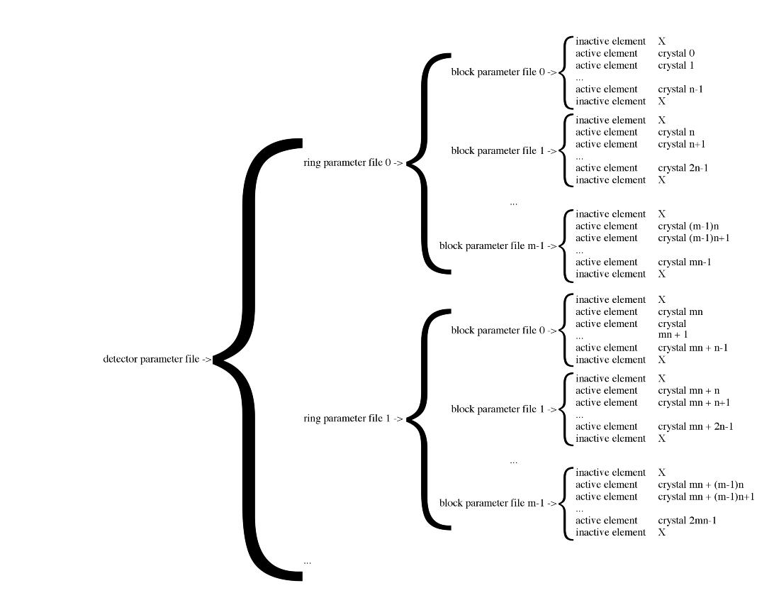
SimSET gives each crystal (actually each block element for which block_material_is_active = TRUE in the block parameter file - a crystal in most tomographs) a number. The crystals are numbered consecutively starting with 0 as the detector parameter file and its component ring and block files are read in: crystal 0 will be the first active element listed in the block parameter file listed first in the ring parameter file listed first in the detector parameter file (figure 1). Note that this will not be the crystal numbering used in a typical tomograph sinogram: the crystals within a block will be numbered consecutively even though they may come from multiple axial rows of crystal within the detector, which a tomograph would sort into separate axial rings of data. It is the user's responsitibilty to re-sort the crystal bins as appropriate. (We considered how this might be done by SimSET, but the flexibility of the block module makes it difficult. The blocks in a ring do not have to be given in any particular order, do not need to have the same crystal layout, and can even have radial layers. If you have an idea of how to approach this, feel free to share it with us - or, even better, write a utility program that will rebin the crystals appropriately!)
Figure 1: The crystal numbering scheme for block detectors. Active block elements are given consecutive numbers starting with 0 as they are read in. Inactive block elements are skipped.
PET coincidences are binned into a number_of_crystals * number_of crystals array. Only the upper triangular portion of the array is used, that is to say a coincidence between crystal A and crystal B is binned into bin (A,B) if B>A (where the second index is the faster varying), bin (B,A) otherwise. The array is not compressed, however.
To activate binning by crystal, include the following line in the binning parameters file:
BOOL bin_by_crystal = true
Crystal binning can be combined with any of the other binning options (e.g., scatter state, energy), though this is somewhat redundant in some cases (i.e., the other line-of-response binning options).
[top of page] [example binning parameter files]
Adding time-of-flight to projections:
Time-of-flight binning is only available for PET simulations.
SimSET keeps track of the total distance photons travel, from their creation to their last interaction in the detector. From this SimSET calculates the time-of-flight (TOF) difference between two coincidence photons from this travel distance. The TOF difference allows the annihilation position of the coincidence photons along the line-of-response to be computed, though the calculation is not particularly accurate due to imperfect time resolution in the detection process (modeled in the detector module).
The binning module includes an option to bin the TOF difference between coincident photons. The user specifies the number of TOF bins, and the minimum and maximum acceptable TOF differences in nanoseconds - coincidences between photons with a TOF difference outside this range are discarded. For example:
INT num_tof_bins = 32
REAL min_tof = -2.541
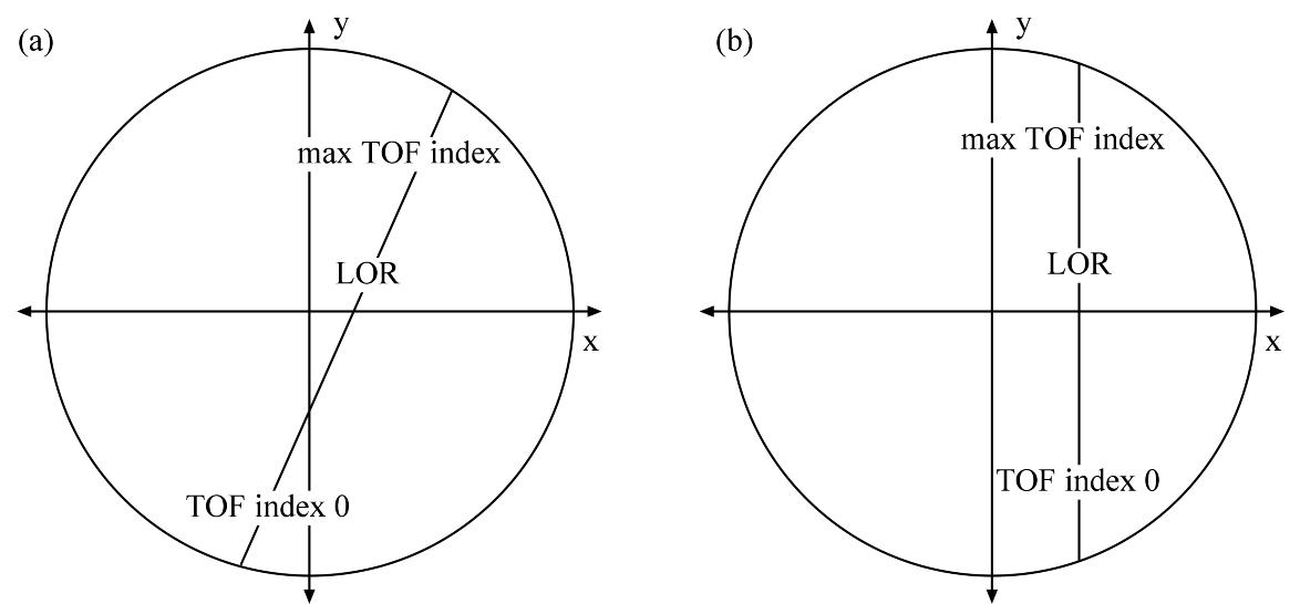
REAL max_tof = 2.387The index increases in the positive x direction, i.e., TOF bin 0 is on the -x side of the line-of-response (LOR) between the detected position of the two photons, the maximum TOF bin is on the +x side (figure 2a). In the event that the line is vertical, then the detected y position is used to orient the line (figure 2b).
Figure 2: (a) The TOF index increases in the direction of increasing x. (b) If the line of response (LOR) is vertical, then the TOF index increases in the direction of increasing y.
TOF binning can be combined with any of the other PET binning options (e.g., scatter state, energy, line-of response).
[top of page] [example binning parameter files]
Output file specification
To avoid creating any one of the following output files, supply an empty string ("") in the relevant "_path" parameter or omit the line entirely.
Set 'add_to_existing_img' to TRUE to add binning results to existing histogram files.
Set 'count_image_path' to the file name to contain the raw counts data. The count image contains the number of decays simulated. If no importance sampling has been used the values in this histogram will be proportional to the estimated count rate. If importance sampling has been used, then this data will contain bias. It may nevertheless be useful for validation purposes.
Set 'count_image_type' to specify the data type used for each voxel:
count_image_type = 0 for one byte integers
count_image_type = 1 for two byte integers
count_image_type = 2 for four byte integersSet 'weight_image_path' to the file name to contain the voxel weights. The weight image is a histogram containing the sums of the weights for each simulated photon. The values in each element are proportional to the mean estimated count rate, whether or not importance sampling has been used.
Set 'weight_image_type' to specify the data type used for each voxel:
weight_image_type = 2 for four byte reals
weight_image_type = 3 for 8 byte realsSet 'weight_squared_image_path' to the file name to contain the weights-squared image. This is a map of the variance of the estimated mean count-rates, accounting for the effects of importance sampling. The data type does not need to be specified as it is always the same as the weight image.
[top of page] [example binning parameter files]
Run-time precision
Control over the run-time precision of the summing of weights during histogram creation is obtained by setting the parameter 'sum_according_to_type' TRUE or FALSE. Setting this parameter TRUE causes the summation to occur using the same precision as that specified for the output data files. Setting it FALSE causes the summation to occur using double-precision REALS and/or 4-byte INTEGERS. If the specified output precision is less than this, the values are converted "down" when the output is written.
The RAM requirement for the summation buffers can become very large, particularly for PVI or DHCI. Setting 'sum_according_to_type' to TRUE may compromise accuracy (to a degree which depends on the exact situation), but can reduce the RAM requirement to a more manageable level.
[top of page] [example binning parameter files]
Estimating mean, variance, and number of counts from SimSET data
SimSET offers three ways to bin data: the number of counts in each bin, the sum of the photon or coincidence weights in each bin, and the sum of the squares of the weights.
When no importance sampling is used (e.g., no stratification, forced detection, or forced non-absorption in the PHG, no forced interaction in the detector module, and no SPECT collimation), the count data can be used in the same way as normal nuclear medicine data--the number of counts in a bin can be used to estimate the mean and variance of the number of counts that would be seen in that bin in an average realization. However, the weight data is still necessary if you really want to simulate a study with the specified activity and scan duration. The number of counts will vary proportionally with the number of decays simulated (num_to_simulate in the run file); the weights, however, use the activity and duration to calculate how many 'real-world' decays each simulated decay represents. (Though, as we don't currently simulate specific isotopes, we are assuming a 100% branching ratio for production of the specified decay product, i.e. either positrons or photons of the specified energy. The specified activity should be adjusted by the branching ratio when this is not true.)
Thus the weights are the best estimate of the mean number of counts in each bin for a study with the specified activity and duration. This true even when importance sampling is used, indeed, the counts cannot be used to estimate the mean in this case. When using weights, the variance is estimated by the sum of the squares of the weight.
When using weights, the question often arises, "How many counts in a real-world study is this simulation equivalent to?", i.e., how do we compare the variance of SimSET data with the variance of a scan?
SimSET computes a quality factor for the binned data from each run. It is reported in the screen output of the run along with the total accepted counts, weights, and sum of squared weights. Here are the appropriate lines from a sample output file:
Total accepted coincidences in this simulation = 3710708
Sum of accepted coincidence weights in this simulation = 1.630578e+07
Sum of accepted coincidence squared weights in this simulation = 1.133462e+08
Quality factor in image data = 6.32e-01
The quality factor, Q, is a number between 0 and 1 that estimates how many real-world events each simulated event is worth in terms of variance.
Q = (sumw)^2 / (N *sumwsq)
where N is the number of counts, sumw is the sum of the weights, and sumwsq is the sum of the squared weights. If we wanted to estimate how many counts, C, would be needed in a scan to achieve approximately the same variance as the simulation above, we would compute C as
C = Q * N = 0.632 * 3710708 = 2345167
Thus the simulation is approximately equivalent to a 2.3 million event scan.
A more rigorous treatment of these issues can be found in (Haynor et al 1991)
Parameter type definitions for binning parameter files
Parameter name Units Data type Binning by photon energy:
num_e_bins
INT min_e keV REAL max_e keV REAL Binning by scatter/randoms:
accept_randoms BOOL scatter_random_param
INT.
possible values:
0 combine primaries, scatters, and randoms 1 single index with two bins, one for all the non-scattered events (for PET this will include randoms where neither photon has scattered, if accept_randoms is true) and one with all events with one or more scatters (a PET coincidence is binned as scatter if either photon has scattered) 2 bin by number of scatters into (max_s-min_s)+1 bins for SPECT, ((max_s-min_s)+1)*((max_s-min_s)+1) bins for PET (each photon has a separate index). Photons with scatter counts below min_s or above max_s are discarded. 3 same as scatter_random_param = 2 except that photons with scatter counts >= max_s are histogrammed into the maximum index value rather than discarded. 4 (PET-only) to histogram coincidences into one index with (max_s-min_s)+1 bins using (blueScatters + pinkScatters) to compute the index number. The coincidence is rejected if the sum is < min_s or > max_s. 5 (PET-only) is the same as scatter_random_param = 4 except that coincidences with (blueScatters + pinkScatters)>= max_s are histogrammed into the top index rather than discarded. (6-10) (PET-only) scatter_random_param from 6-10 are the same as 1-5 except that randoms are histogramed separately into an extra bin. The randoms bin is always the last bin. For options where the two photons are each given their own index (i.e., scatter_random_param = 6 or 7), the two photon indices are combined into a single linear index with one extra bin at the end for the randoms. 6 (PET-only) to have three bins: one for true unscattered coincidences, the second for non-random scattered coincidences, the third for random coincidences. 7 (PET-only) to have the same binning as scatter_random_param = 2 except with an extra bin for randoms, i.e., non-random coincidences are binned as with 2, but all random coincidences are binned separately to an extra bin at the end of the array. 8 (PET-only) to have the same binning as scatter_random_param = 3 except with an extra bin for randoms, i.e., non-random coincidences are binned as with 3, but all random coincidences are binned separately to an extra bin at the end of the array. 9 (PET-only) to have the same binning as scatter_random_param = 4 except with an extra bin for randoms, i.e., non-random coincidences are binned as with 4, but all random coincidences are binned separately to an extra bin at the end of the array. 10 (PET-only) to have the same binning as scatter_random_param = 5 except with an extra bin for randoms, i.e., non-random coincidences are binned as with 5, but all random coincidences are binned separately to an extra bin at the end of the array. min_s
INT max_s
INT Sinogram binning:
num_z_bins
INT min_z cm REAL max_z cm REAL do_msrb
BOOL do_ssrb
BOOL detector_radius cm REAL num_aa_bins
INT num_td_bins
INT min_td cm REAL max_td cm REAL 3D-RP binning:
num_phi_bins
INT num_theta_bins
INT max_theta degrees REAL num_xr_bins
INT min_xr cm REAL max_xr cm REAL num_yr_bins
INT min_yr cm REAL max_yr cm REAL Crystal (pair) binning:
bin_by_crystal
BOOL Time-of-flight binning:
num_tof_bins
INT min_tof nanoseconds REAL max_tof nanoseconds REAL Output file specification:
add_to_existing_img
BOOL weight_image_type
INT.
possible values:
2 four-byte reals 3 eight-byte reals count_image_type
INT.
possible values:
0 one-byte integers 1 two-byte integers 2 four-byte integers weight_image_path
STR weight_squared_image_path
STR count_image_path
STR Binning history file:
history_file
STR
Allows the creation of a history file of photons which pass the binning criteria (see history files page)history_params_file
STR
Configures history file creation for photons which pass the binning criteria (see history files page)Summation precision:
sum_according_to_type
BOOL
Binning is usually performed 'on-the-fly' during simulation. However, it is also possible to use the binning module on pre-existing history files. This process is achieved using the PhgBin utility (see Utilities page). PhgBin takes a phg run-time parameter file as input. It then reads the specified history file and re-bins it according to the criteria specified in the bin_params file.
NOTE: PhgBin only works on standard (non-customized) history files. See the History files chapter for information on post-processing of customized history files
To use the binning module you can copy the file "bin_params" which is supplied with the SimSET package. This is a simple text file which you can edit to specify your binning needs.
-Sinogram example
-3D-RP example
Last revised by: Robert Harrison Revision date: 4 March 2009