|
 |
|
|
Supported models
The Detector module receives photons either directly from the PHG module or from the Collimator module. It tracks photons through the specified detector, recording the interactions within the detector for each photon. The interactions are used to compute a detected location and total energy deposited. Gaussian energy blurring may be applied. The clickable diagram above depicts the four currently supported detector types: planar (SPECT), dual head coincidence (PET), cylindrical (PET), and block (PET and SPECT) detector models are currently supported, together with a 'simple' model in which only the Gaussian energy blurring is performed.
Outputs
Detected Photon Data is passed from the detector module to either the binning module or the history file module depending on the options specified in the PHG Parameter File. This data includes total deposited energy, energy weighted centroid for planar and cylindrical detectors or detected crystal number for block detectors, list of interaction positions and energy deposited, and detected position.
Importance sampling
To increase the efficiency of the detector module an importance sampling feature, forced-interaction, is provided. Forced-interaction causes every photon impinging on the first layer of the detector to undergo at least one interaction. The photon weight is adjusted to avoid bias (see Haynor et al, 1991). We suggest that you test this option for a given detector system before using it for longer runs: in some complex detector systems, particular in complex block detector systems, it can slow simulations significantly. It provides the greatest detection efficiency gains in systems where photons are likely to pass through the detectors without interacting (e.g., animal PET systems with 10mm crystals or thin-crystal SPECT systems); it slows simulations down when photon paths can intersect many different detector elements in a complex detector system.
Customization
Each detector model allows the user to write a User Routine to modify the behavior of the detector software. The detector parameters and the current photon and decay structures are provided to the user routine. It is called before the detector code models the transport through the detector. The user routine may modify any parameter of the current photon or have it rejected by the detector module. To customize the detector simulation, modify the 'dummy' detector module user routine with user code (DetUsr.c) and re-build PHG software. Photon and decays can also be modified immediately after the detector module and before further processing at the beginning of the binning module (see PhgUsrBin.c) or, if randoms are being simulated, at the beginning of the randoms processing module (see addRandUsr.c).
[top of page] [physical models] [configuring detector models] [example parameter files]
Planar SPECT
Detector model
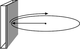
The Planar SPECT (or "flat detector") mode provides a full simulation (including scatter, absorption, and penetration) of gamma photon transport in a planar detector.
Figure 1. Example Planar SPECT simulation: 2-layer flat detector with collimator
The detector is modeled as layered rectangular parallelepipeds (see figure 1). Each layer can be specified as active or inactive. Photon transport is identical in active and inactive layers, however only interactions within active layers are used for the computation of centroid and total deposited energy (see figure 2). This allows layers of graded absorber (inactive), detector housing (inactive), and crystal materials (active) to be simulated. X-ray fluorescence photons, scintillation photons and photomultiplier tubes are not simulated.
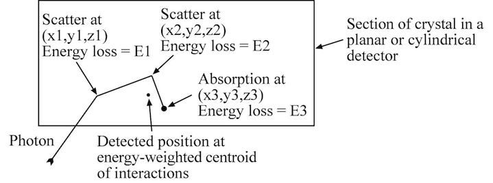
Figure 2. Detected energy and position for planar and cylindrical detectors. A photon's detected energy is calculated as the sum of the energy deposited for all interactions in active (e.g. scintillating) elements of the detector. The detected position is calculated as the energy-weighted centroid of these interactions. The Flat Detector can be rotated through any angular range at a fixed radius, stopping at a user specified number of locations (views), or can be continuously rotated. The radial and axial position of the detector is predetermined by the collimator module.
Photon modeling and forced interaction
Incoming photons are projected to the surface of the detector, and then tracked using the same method as applied in the object (this will be documented in the Physics and Algorithms page). If forced interaction is selected, a photon that impinges on the first layer of the detector undergoes the following:
- The photon path is projected through the detector to calculate the total attenuation path-length
- An interaction point is randomly selected from the truncated exponential distribution within the detector
- The photon's weight is adjusted to reflect the probability that the interaction would have occurred
- The photon's position is updated to the new location and an interaction is simulated
After the first interaction no further forced-interactions are performed.
The location and deposited energy are recorded for each interaction. When the photon escapes or is absorbed, an energy weighted centroid and total deposited energy are computed.
Outputs
In addition to the output supplied by the PHG, the Flat Detector software provides statistics on the following:
- The number of photons passed to the detector module
- The number of photons reaching the first layer
- The number of photons depositing energy in the detector
- The number of photons absorbed in the detector
- The total photon weight absorbed in the detector
- The number of photons absorbed on the first interaction
- The total photon weight of first-interaction absorptions
- The number of photons passing through without interacting
- The number of photons absorbed due to reaching the maximum interaction number (a program constant set in Photon.h)
[top of page] [physical models] [configuring detector models] [example parameter files]
Dual Headed (DHCI) PET
Detector and photon modeling
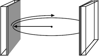
This mode provides a full simulation (including scatter, absorption, and penetration) of coincidence detection using two planar detectors separated by 180 degrees. The modeling of photon transport through the detectors is the same as described in the Planar SPECT section above. In fact, DHCI simulation is performed using the flat detector software, and all the options available with flat detectors are available for DHCI, including multiple layers of different materials and multiple detector positions. For each decay, the detector position is randomly selected from the user-specified range.
Outputs
As with the Flat Detector software, the DHCI software provides statistics on the following:
- The number of photons passed to the detector module
- The number of photons reaching the first layer
- The number of photons depositing energy in the detector
- The number of photons absorbed in the detector
- The total photon weight absorbed in the detector
- The number of photons absorbed on the first interaction
- The total photon weight of first-interaction absorptions
- The number of photons passing through without interacting
- The number of photons absorbed due to reaching the maximum interaction number (a program constant set in Photon.h)
However, these outputs are modified to include statistics for both blue and pink photons (see photon history files page) rather than just single photon statistics.
[top of page] [physical models] [configuring detector models] [example parameter files]
Cylindrical PET
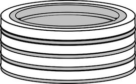
Figure 4. Example cylindrical PET simulation: 2-layer cylindrical detector.
Detector model
The cylindrical detector software can be used to simulate 2D and 3D PET (PVI): for most tomographs the cylindrical detector model is not as exact as the block detector model (see below), but it is a reasonable approximation for many investigations. The cylindrical detector software models the detector as a series of adjacent regular right cylinders with transaxial layers (see figure 4). Photon interactions including scatter, absorption, and penetration are simulated, but there are no blocks and hence no gap effects.
The cylindrical detector software may also be used to simulate single event rates for PET scans.
The operational principles for the cylindrical detector are very similar to those of the flat detector software. Each detector layer can be specified as active or inactive. Photon transport is identical in active and inactive layers, however only interactions within active layers are used for the computation of centroid and total deposited energy. This allows layers or rings of septa (inactive), detector housing (inactive), and crystal materials (active) to be simulated.
Photon modeling
Incoming photons are projected to the surface of the detector, and then tracked using the same method as applied in the object (this will be documented in the Physics and Algorithms page). If forced interaction is selected, a photon that impinges on the first layer of the detector undergoes the following:
- The photon path is projected through the detector to calculate the total attenuation path-length
- An interaction point is randomly selected from the truncated exponential distribution within the detector
- The photon's weight is adjusted to reflect the probability that the interaction would have occurred
- The photon's position is updated to the new location and an interaction is simulated
After the first interaction no further forced-interactions are performed.
The location and deposited energy are recorded for each interaction. When the photon escapes or is absorbed, an energy weighted centroid and total deposited energy are computed.
Outputs
The cylinder software provides statistics on the following quantities:
- The number of photons passed to the detector module
- The number of coincidence pairs accepted by the detector
- The number of photons depositing energy in the detector
- The number of photons completely absorbed within the detector
- The sum weight of photons completely absorbed within the detector
- The number of photons reaching the first layer
- The number of photons depositing energy in the detector
- The number of photons absorbed in the detector
- The total photon weight absorbed in the detector
- The number of photons forced to interact in the detector
- The total photon weight forced to interact in the detector
- The number of photons absorbed on the first interaction
- The total photon weight of first-interaction absorptions
- The number of photons passing through without interacting
These outputs include statistics for both blue and pink photons (see photon history files page).
[top of page] [physical models] [configuring detector models] [example parameter files]
Block Detector PET or SPECT
Figure 5. Example block detector : at left a single ring composed of 16 blocks of two different types; at right a tomograph composed of three copies of the ring, with the middle ring rotated by 45 degrees.
Detector model
The block detector software is intended for simulation of typical PET block detector systems, though it can also be used for SPECT simulations. The tomograph is modeled as a collection of right rectangular blocks arranged within axial rings (see figure 5). SimSET allows for considerable flexibility in the geometry of block-detector systems. The four main limitations are (1) all elements of the detector system are outside an elliptical cylinder containing the object being imaged, (2) the elements of the detector system be composed entirely of right-rectangular boxes, (3) the axial faces of the blocks are parallel to the x-y plane, and (4) all blocks within an axial ring must have the same axial extent as the ring. The second constraint does not allow for the simulation of triangular cross-section objects, as might be desired for interblock septa; these would need to be approximated as a collection of right-rectangular boxes. The third constraint would, for example, rule out a spherical system, in which the detectors focused on the origin. The fourth contraint rules out systems in which the blocks are staggered axially (see figure 6a); however, such a system could be modeled by splitting the blocks into multiple rings axially (see figure 6b).
Figure 6. (a) The restriction that all blocks in a ring must have the same axial extent rules out this ring, with detectors that are staggered axially. (b) However, this system can be realized by splitting the staggered ring into three abutting axial rings (shown here 'exploded' axially). The blocks themselves may be subdivided by planes parallel to the faces of the block (see figure 7).
Figure 7. A block is a right-rectangular box which can be further subdivided into right-rectangular boxes. Here we show two possibilities: Block A, an interblock septa of tungsten; and Block B, a module of BGO detectors with aluminum front and back plates and tungsten side housing. Within the blocks, photon interactions including scatter, absorption, and penetration are simulated. The space between the blocks is simulated as vacuum, i.e., when outside the blocks, photons are projected to the next block on their path.
Most operational principles for the block detectors are very similar to those of the flat detector software, but the computation of detected energy and position have been changed. As in the planar detector, each detector element can be specified as active or inactive with photon transport identical in active and inactive blocks, and only interactions within active blocks are considered when when calculating detected energy and position. However, energy is totaled by block, and only those interactions in the block with the highest deposited energy are used to compute the detected energy and position:
- Compute energy deposited in the active elements of each block.
- Choose the block with the highest deposited energy.
- Sum only the interactions in the chosen block to compute detected energy.
- Apply energy resolution blurring if set by user.
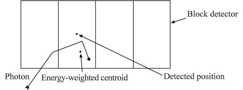
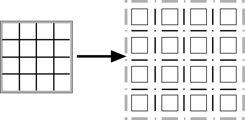
Figure 8. Detected position and crystal calculation for block detectors. In block detectors an energy-weighted centroid (see figure 2) is determined using the interactions in the block with the highest total energy deposited. The detected position is set to the center of the crystal containing the centroid (or the crystal center nearest to the centroid if it is between crystals). After summing the energy in the chosen block, the position is determined using the interactions in this block (see figure 8). There are two built-in options for the final position
- Compute an energy-weighted centroid of the interactions.
- Find the crystal center within the block to which the centroid is closest.
- Set the detected position to the center of this crystal.
- if (blocktomo_position_algorithm = snap_centroid_to_crystal_center) # this is the default
- Set the detected crystal number to the current crystal number. For the crystal numbering scheme, see Binning by crystal pair on the Binning page of the User Guide.
- else # that is if (blocktomo_position_algorithm = use_energy_weighted_centroid), the only other option currently
- Set detected position to the energy-weighted centroid (NOTE that this may be in an inactive element of the block, e.g. in teflon tape between crystals).
These algorithms for detected energy and position may be too simple for your tomograph simulation. If so, you can modify them easily in one of the user functions - examples are given in the User Functions page.
Photon modeling
Incoming photons are projected to the surface of the detector, and then tracked using the same method as applied in the object (this will be documented in the Physics and Algorithms page). If forced interaction is selected, a photon that impinges on the first layer of the detector undergoes the following:
- The photon path is projected through all detectors in its path to calculate the total attenuation path-length
- An interaction point is randomly selected from the truncated exponential distribution within the detectors
- The photon's weight is adjusted to reflect the probability that the interaction would have occurred
- The photon's position is updated to the new location and an interaction is simulated
After the first interaction no further forced-interactions are performed - the photon is tracked normally.
The location and deposited energy are recorded for each interaction. When the photon escapes or is absorbed, an energy weighted centroid and total deposited energy are computed.
Outputs
The block detector software provides statistics on the following quantities:
- The number of photons passed to the detector module
- The number of photons depositing energy in the detector
- The number of photons completely absorbed within the detector
- The sum weight of photons completely absorbed within the detector
- The number of photons forced to interact in the detector (if forced interaction is used)
- The total photon weight forced to interact in the detector (if forced interaction is used)
- The number of photons absorbed on the first interaction
- The total photon weight of first-interaction absorptions
- The number of photons passing through without interacting
- Total weight decremented during forced interaction (if forced interaction is used)
These outputs include statistics for both blue and pink photons (see photon history files page).
[top of page] [physical models] [configuring detector models] [example parameter files]
Activating Detector Modeling
The detector module uses a parameter file format to select the detector model, define detector parameters, and select simulation options. To activate detector modeling:
1. Create a detector parameters file. Entries in this file have the following format:
DATA_TYPE parameter_name = value For example,
REAL reference_energy_keV = 511.0 More detailed information on parameter file formats can be found in Appendix VI. Data type definitions for detector parameter files may be found below in the sections for each detector type.
2. Set 'STR detector_params_file' in the PHG run-time parameters file to this file's pathname.
3. Create the following entries in the detector parameters file:Set 'STR history_params_file' to name of history parameters file if one is to be used. Leave blank if no history file is being created.
Set 'STR history_file' to the name of the history file (if one is to be used)
Set 'history_file' to the desired name of the new history file. Only photons and detection records accepted by the detector module are written to this history file. It must have a different name from any other history files specified in the simulation (such as from the phg run-time parameters or elsewhere). Leave blank for no history file creation.
Set 'do_forced_interaction' to true or false.Set 'ENUM detector_type' to desired model:
simple_pet - Apply Gaussian blurring to the incident energy only simple_spect - Apply Gaussian blurring to the incident energy only planar - Monte Carlo simulation of flat detectors for SPECT dual_headed - Monte Carlo simulation of PET imaging using two opposing planar detectors cylindrical - Monte Carlo simulation of PET imaging using a cylindrical detector block - Monte Carlo simulation of PET imaging using block detectors To Gaussian blur the total energy deposited:
Set 'REAL reference_energy_keV' to starting photon energy
Set 'REAL energy_resolution_percentage' to FWHM percent energy resolution
The remaining detector parameters depend on the detector type chosen:
- Configuring Planar SPECT
- Configuring DHCI PET
- Configuring Cylindrical PET
- Configuring Block PET or SPECT
No further parameters are required if simple_pet or simple_spect detectors have been selected.
[top of page] [physical models] [configuring detector models] [example parameter files]
Configuring Planar SPECT
(See figure 9 below for illustration of some of the following variables.)
Set 'INT plnr_num_layers' to the desired number of detector layers.
Set 'REAL plnr_inner_radius' to the inner radius of the detector rotation (see figure 9).
Set 'REAL plnr_transaxial_length' to the transaxial length of the detector (see figure 9).
Set 'REAL plnr_axial_length' to the axial length (height) of the detector (see figure 9).For a rotating gamma camera, set 'REAL plnr_min_angle' to the start position and set 'REAL plnr_max_angle' to the stop position (in degrees).
Set 'INT plnr_num_views' to the number of angular locations at which the detector is positioned.NOTE: If the Collimator Module is being used, this number must match the number of views specified in the Collimator Parameters File.
NOTE: Set plnr_num_views to -1 for continuous rotation. For continuous rotation plnr_min_angle must be 0 and plnr_max_angle must be 180 for SPECT, 360 for DHCI.
For no rotation, set 'REAL plnr_min_angle' and 'REAL plnr_max_angle' to the same value.
For each layer (starting with the inner layer)
- Set 'NUM_ELEMENTS_IN_LIST plnr_layer_info_list' to 3.
- Set ''REAL plnr_layer_depth' to the radial depth of the layer (see figure 9).
- Set 'INT plnr_layer_material' to the index of the desired layer material in the attenuation table.
- Set 'BOOL plnr_layer_is_active' to true for scintillating materials, false for non-scintillating materials.
Figure 9. Parameters for planar detectors.
[top of page] [physical models] [configuring detector models] [example parameter files]
Configuring Dual Head PET
Set 'BOOL simulate_PET_coincidences_only' or 'BOOL simulate_PET_coincidences_plus_singles' to true in PHG Parameters File. This forces simulation of PET.
Set 'INT plnr_num_layers' to the desired number of detector layers.
Set 'REAL plnr_inner_radius' to the inner radius of the detector rotation (see figure 9).
Set 'REAL plnr_transaxial_length' to the transaxial length of the detector (see figure 9).
Set 'REAL plnr_axial_length' to the axial length (height) of the detector (see figure 9).
The possible detector positions are determined from the parameters 'plnr_min_angle', 'plnr_max_angle', and 'plnr_num_views'.
Set ''REAL plnr_min_angle' to the minimum angular position (degrees) of the detector rotation (see figure 10).
Set ''REAL plnr_max_angle' to the maximum angular position (degrees) of the detector rotation (see figure 10).
Set ''REAL plnr_num_views' to the number of detector positions (stops) between plnr_min_angle and plnr_max_angle (see figure 10).
Currently the first detector position is centered on plnr_min_angle. A feature to enable half-bin offsetting is currently being implemented. This feature will be controlled by setting 'first_angle_offset' to true or false (see figure 10).The last collimator position will then be centered at (plnr_min_angle - one bin) or (plnr_max_angle - one half bin) respectively. (Not implemented as of Feb 10th 2009)
Figure 10. Detector positions for DHCI PET. Note: first_angle_offset feature not yet implemented for DHCI.
For each layer (starting with the inner layer)
- Set 'NUM_ELEMENTS_IN_LIST plnr_layer_info_list' to 3.
- Set 'REAL plnr_layer_depth' to the radial depth of the layer (see figure above).
- Set 'INT plnr_layer_material' to the index of the desired layer material in the attenuation table.
- Set 'BOOL plnr_layer_is_active' to true for scintillating materials, false for non-scintillating materials.
Parameter type definitions for planar detector parameter files
Parameter name Units Data type history_file
STR
Allows the creation of a history file of photons processed by the detector module (see history files page)history_params_file
STR
Configures history file creation for photons processed by the detector module (see history files page)do_forced_interaction
BOOL detector_type
If text, then ENUM, else INT. Options shown below:
ENUM INT simple_pet 1 simple_spect 2 reserved 3 reserved 4 planar 5 cylindrical 6 dual_headed 7 block 8 reference_energy_keV keV REAL energy_resolution_percentage
REAL plnr_num_layers
INT plnr_inner_radius cm REAL plnr_transaxial_length cm REAL plnr_axial_length cm REAL plnr_min_angle degrees REAL plnr_max_angle degrees REAL plnr_num_views
INT plnr_layer_info_list
NUM_ELEMENTS_IN_LIST plnr_layer_depth cm REAL plnr_layer_material
INT plnr_layer_is_active
BOOL first_angle_offset degrees BOOL
[top of page] [physical models] [configuring detector models] [example parameter files]
Configuring Cylindrical PET
Cylindrical detectors systems are continuous axial rings of detectors or other materials. Each ring may be split into layers of different material radially. Within each ring/layer there are no material changes or gaps.
To define a cylindrical detector, set the following fields in the detector parameters file:
(0) Detector type
(1) Forced interaction, true or false
This is an importance sampling feature that forces every photon to interact in the crystal--no photons escape without interaction.
(2) Number of rings
(3) For each ring
(3.0) Set cyln_ring_info_list = number of layers in this ring + 3
This is counter the program uses to keep track of how many entities it needs to read in for this ring. It must read in the axial minimum and maximum, the number of layers, and a list of parameters for each layer.
(3.1) Axial minimum
(3.2) Axial maximum
(3.3) Number of layers
(3.4) For each layer
(3.4.0) Set cyln_layer_info_list = 4
This is counter the program uses to keep track of how many entities it needs to read in for this layer.
(3.4.1) Layer material
(3.4.2) Layer inner radius
(3.4.3) Layer outer radius
(3.4.4) Layer active or inactive
For most tomographs this can be interpreted as meaning scintillating or non-scintillating: the crystal will be active, any crystal housing or structufral ellements will be inactive. Anywhere that deposited energy will contribute to the detected energy/position of the photon should be defined as active.
(4) Specify an energy resolution (energy blurring) if desired:
(4.1) Specify the reference energy in keV
(4.2) Specify the percent full-width half maximum for the Gaussian blurring
(5) (Not yet an official feature) Specify a photon time-of-detection resolution if desired:
(5.1) Specify the full-width half maximum for the Gaussian blurring in nanoseconds.
Each photon will have its detected time 'blurred' by a Gaussian with this FWHM. The time-of-flight resolution will be sqrt( 2 * FWHM * FWHM ) as both photons in a coincidence have their energy blurred.
(6) Specify a history file, if desired.
(6.1) Specify custom history file parameters if desired
[top of page] [physical models] [configuring detector models] [example parameter files]
Parameter type definitions for cylindrical detector parameter files
| Parameter name | Units | Data type | ||||||||||||||||||
| do_forced_interaction | BOOL | |||||||||||||||||||
| detector_type | If text, then ENUM, else INT. Options shown below:
|
|||||||||||||||||||
| cyln_num_rings | INT | |||||||||||||||||||
| cyln_ring_info_list | INT | |||||||||||||||||||
| cyln_num_layers | INT | |||||||||||||||||||
| cyln_min_z | cm | REAL | ||||||||||||||||||
| cyln_max_z | cm | REAL | ||||||||||||||||||
| cyln_layer_material | INT | |||||||||||||||||||
| cyln_layer_inner_radius | cm | REAL | ||||||||||||||||||
| cyln_layer_outer_radius | cm | REAL | ||||||||||||||||||
| cyln_layer_is_active | BOOL | |||||||||||||||||||
| reference_energy_keV | keV | REAL | ||||||||||||||||||
| energy_resolution_percentage | REAL | |||||||||||||||||||
| photon_time_fwhm_ns | ns | REAL | ||||||||||||||||||
| history_file | STR Allows the creation of a history file of photons processed by the detector module (see history files page) |
|||||||||||||||||||
| history_params_file | STR Configures history file creation for photons processed by the detector module (see history files page) |
[top of page] [physical models] [configuring detector models] [example parameter files]
Definition of a block-detector system requires three levels of parameter files: parameter files describing the block type or types used; parameter files arranging blocks into rings (or other arrangements, as long as they fit inside two nested elliptical cylinders); and a parameter file which creates a tomograph from a stack of rings and defines some general tomograph parameters.
All distances in the parameter files are measured in cm, all angles in degrees.
The parameter files to define a typical commercial PET system are many thousand lines long in total. The ring parameter files are particularly long. To facilitate input of these files, we are providing MatLab programs for defining the ring and block parameters. We would also be interested in similar programs in C or using an open source package (e.g., FreeMat) - if a user would like to write one!
Defining the blocks
The basic unit for a block-detector system is the block. Blocks are right-rectangular boxes. Blocks are further subdividable into smaller right-rectangular boxes.
First we set reference point coordinates for the block: these are somewhat arbitrary, but the ring parameters (described below) use this point to position the block within the ring and as a pivot point when orienting the block. The reference point is set with the parameters 'REAL block_reference_x', 'REAL block_reference_y' and 'REAL block_reference_z'.
Next we set the extent of the block in the x (radial depth, for the default block orientation in the ring), y (transaxial width), and z (axial height) directions. We set these with the parameters 'REAL block_x_minimum' and 'REAL block_x_maximum', 'REAL block_y_minimum' and 'REAL block_y_maximum', and 'REAL block_z_minimum' and 'REAL block_z_maximum'. The reference point must fall within the range of these parameters. (These ranges and the x and y directions are 'relative' to the reference point, as blocks may be shifted and rotated when positioning them in a ring, as described in the next section. See figure 11.)
Figure 11. The user first defines some general characteristics of the block: a reference point (here the point at the middle of the front face of the block); the range of values the block occupies in the x, y and z dimensions; and the number of layers. Each block has its own coordinate system, with x corresponding to the depth into the block (the radial direction, for the default block orientation in the tomograph), y corresponding to the other transaxial dimension, and z corresponding to the axial dimension.
Blocks can be split into layers in the x-direction. Each layer can then be subdivided into non-uniform elements at user-specified boundaries in the y and z direction. Layers extend across the entire block, and the other boundaries extend across the entire layer, thus some parts of the block (e.g. the housing) will be defined as multiple voxels (figure 12).
Figure 12. All material boundaries are extended across the whole block. Here a block layer consisting of detector housing, crystals, and inter-crystal gaps is split into the elements that would need to be defined in the block parameter file.
The user specifies the number of layers in a block using 'INT block_num_layers N', where N is the desired number. Then the parameter 'NUM_ELEMENTS_IN_LIST block_layer_info_list' gives the number of componenets in the list describing a block layer and should be set to 5.
The first two list components are for parameters 'REAL block_layer_inner_x' and 'REAL block_layer_outer_x', which give the radial extent of the current layer. (Note the block_layer_inner_x of the first layer must be block_x_minimum and the block_layer_outer_x of the last layer must be block_x_maximum.) The other three list components for the layer are sub-lists giving the positions and composition of the elements in the layer. 'NUM_ELEMENTS_IN_LIST block_layer_num_y_changes' gives the layer's number of material changes in the y direction. It is followed by a sub-list giving the y-value for each of those boundaries, 'REAL block_layer_y_change'. Similarly 'NUM_ELEMENTS_IN_LIST block_layer_num_z_changes' gives the number of changes in the z direction and is followed by a sub-list of 'REAL block_layer_z_change' giving the z-boundaries. (For instance, in figure 12 there are 9 elements in each direction, thus block_layer_num_y_changes and block_layer_num_z_changes would both be 8; the lists for block_layer_y_change or block_layer_z_change would give the y or z coordinate for each of the boundaries .)
The final sub-list in the layer definition gives the composition of each of the material elements in the layer. The number of elements in this list are given as 'NUM_ELEMENTS_IN_LIST block_layer_material_elements', which must be equal to (block_layer_num_y_changes + 1)*(block_layer_num_z_changes + 1). Each element of this sub-list is a list of the following form:
Parameter type definitions for block parameter files
| Parameter name | Units | Data type |
| block_reference_x | cm | REAL |
| block_reference_y | cm | REAL |
| block_reference_z | cm | REAL |
| block_x_minimum | cm | REAL |
| block_x_maximum | cm | REAL |
| block_y_minimum | cm | REAL |
| block_y_maximum | cm | REAL |
| block_z_minimum | cm | REAL |
| block_z_maximum | cm | REAL |
| block_num_layers | INT | |
| block_layer_info_list | NUM_ELEMENTS_IN_LIST | |
| block_layer_inner_x | cm | REAL |
| block_layer_outer_x | cm | REAL |
| block_layer_num_y_changes | NUM_ELEMENTS_IN_LIST | |
| block_layer_y_change | cm | REAL |
| block_layer_num_z_changes | NUM_ELEMENTS_IN_LIST | |
| block_layer_z_change | cm | REAL |
| block_layer_material_elements | NUM_ELEMENTS_IN_LIST | |
| block_material_info_list | NUM_ELEMENTS_IN_LIST | |
| block_material_index | INT | |
| block_material_is_active | BOOL |
[top of page] [physical models] [configuring detector models] [example parameter files]
Defining the rings
Rings are collections of blocks with common axial extent. The blocks must all be placed between an inner elliptical cylinder and outer elliptical cylinder. Outside of these restrictions, the blocks can be arranged in any non-overlapping arrangement within the ring.
Ring definition starts with definition of the bounding elliptical cylinders. These do not need to be the largest (smallest) cylinders inside (outside) all the blocks. However, the inner cylinder must lay entirely outside the collimator (or object cylinder if no collimator is used). The elliptical cylinders are defined by giving x and y 'radii' (half the length of the major and minor axes) using the parameters 'REAL ring_x_inner_radius', 'REAL ring_x_outer_radius', 'REAL ring_y_inner_radius' and 'REAL ring_y_outer_radius' - for circular cylinders the x and y radii should be equal. The z boundaries of the elliptical cylinders are defined using the parameters 'REAL ring_z_minimum' and 'REAL ring_z_maximum'. The z boundaries are 'relative' - the whole ring may be shifted axially in the block-based tomograph file, as described in the following section. The z-minimums and maximums of all the blocks in the ring must match these ring boundaries (after applying any axial shift given below when positioning them in the ring).
The next parameter defined is the number of blocks in the ring, 'NUM_ELEMENTS_IN_LIST ring_num_blocks_in_ring'. This is then followed by a list of parameters for each of the blocks in the ring. The first parameter declares the length of the list of parameters to follow, 'NUM_ELEMENTS_IN_LIST ring_block_description_list' and is set to 5. The following parameter gives the pathname of the block parameter file to be used, 'STR ring_block_parameter_file'. The remaining four parameters define the position and orientation of the block within the ring: the radial, angular and axial position of the block reference point (defined in the block parameter file) within the ring, 'REAL ring_block_radial_position', 'REAL ring_block_angular_position', and 'REAL ring_block_z_position'; and the transaxial orientation angle of the block in degrees, 'REAL ring_block_transaxial_orientation'. This ring_block_transaxial_orientation (see figure 13) gives a rotation of the block: if it is set to 0, the face of the block is perpendicular to the radial vector from the tomograph axis to the the block reference point, with the block's internal x-coordinate parallel to this radius vector with x increasing with radial position; if it is set to a positive number, the block face is rotated counterclockwise (so that a ring_block_transaxial_orientation of 90 degrees corresponds to the block's internal y-coordinate parallel to the radial vector with y increasing with radial position); if it is set to a negative number, the block face is rotated clockwise (so that a ring_block_transaxial_orientation of -90 degrees corresponds to the block's internal y-coordinate parallel to the radial vector with y decreasing with radial position).
Figure 13. The transaxial block orientation angle is a transaxial rotation of the block using the reference point of the block as a pivot point. If the angle is set to 0, the vector perpendicular to the block face at the reference point will point towards the z-axis. Positive angles correspond to counterclockwise rotations of the block: here a rotation of approximately 30 degrees is shown.
Parameter type definitions for ring parameter files
| Parameter name | Units | Data type |
| ring_x_inner_radius | cm | REAL |
| ring_x_outer_radius | cm | REAL |
| ring_y_inner_radius | cm | REAL |
| ring_y_outer_radius | cm | REAL |
| ring_z_minimum | cm | REAL |
| ring_z_maximum | cm | REAL |
| ring_num_blocks_in_ring | NUM_ELEMENTS_IN_LIST | |
| ring_block_description_list | NUM_ELEMENTS_IN_LIST | |
| ring_block_parameter_file | STR | |
| ring_block_radial_position | cm | REAL |
| ring_block_angular_position | degrees | REAL |
| ring_block_z_position | cm | REAL |
| ring_block_transaxial_orientation | degrees | REAL |
[top of page] [physical models] [configuring detector models] [example parameter files]
Defining the block-based tomograph
A block-based tomograph parameter file defines the tomograph as an axial stack of rings, each of which can be rotated transaxially. In addition to the parameter file gives some general tomograph simulation parameters (the same as those used in other detector simulations).
The general tomograph parameters in the file are: the detector type, 'ENUM detector_type = block'; the pathnames of the detected photon history file, if desired, 'STR history_file' and custom history file format, if any, 'STR history_params_file'; a toggle switch for forced interaction, 'BOOL do_forced_interaction' (note that forced interaction may reduce the efficiency of some block detector simulations - we recommend a short test run to check before setting this feature TRUE with blocks); the energy resolution in percentage full-width-half-maximum (FWHM), 'REAL energy_resolution_percentage', and the reference energy on which the resolution is based, 'REAL reference_energy_keV'; and the time-of-flight (TOF) resolution FWHM for a photon in nanoseconds, 'REAL photon_time_fwhm_ns' (note that for coincidence time difference the TOF resolution will be the squareroot of twice the square of this quantity).
The first block-specific parameter is the number of rings in the tomograph, 'NUM_ELEMENTS_IN_LIST blocktomo_num_rings'. After that follows lists for each of the rings. Each of these lists are prefaced with the parameter 'NUM_ELEMENTS_IN_LIST blocktomo_ring_description_list' which is set to 3, the number of parameters for each ring. Each list consists of three items: the pathname of the ring parameter file, 'STR blocktomo_ring_parameter_file'; an axial shift for placing the ring within the tomograph, 'REAL blocktomo_ring_axial_shift'; and a transaxial rotation (positive numbers connote counterclockwise rotation) for the ring, 'REAL blocktomo_ring_transaxial_rotation'.
Parameter type definitions for block-based tomograph parameter files
| Parameter name | Units | Data type | ||||||||||||||||||
| detector_type | If text, then ENUM, else INT. Options shown below:
|
|||||||||||||||||||
| history_file | STR Allows the creation of a history file of photons processed by the detector module (see history files page) |
|||||||||||||||||||
| history_params_file | STR Configures history file creation for photons processed by the detector module (see history files page) |
|||||||||||||||||||
| do_forced_interaction | BOOL | |||||||||||||||||||
| energy_resolution_percentage | REAL | |||||||||||||||||||
| reference_energy_keV | keV | REAL | ||||||||||||||||||
| photon_time_fwhm_ns | ns | REAL | ||||||||||||||||||
| blocktomo_position_algorithm | ENUM |
One of two options, snap_centroid_to_crystal_center (default) or use_energy_weighted_centroid. See above for algorithmic details. |
||||||||||||||||||
| blocktomo_num_rings | NUM_ELEMENTS_IN_LIST | |||||||||||||||||||
| blocktomo_ring_description_list | NUM_ELEMENTS_IN_LIST | |||||||||||||||||||
| blocktomo_ring_parameter_file | STR | |||||||||||||||||||
| blocktomo_ring_axial_shift | cm | REAL | ||||||||||||||||||
| reference_energy_keV | keV | REAL | ||||||||||||||||||
| blocktomo_ring_transaxial_rotation | degrees | REAL |
[top of page] [physical models] [configuring detector models] [example parameter files]
- Generic contains samples of all types of detectors.
- Planar SPECT detector parameters file.
- DHCI detector parameters file.
- Cylindrical PET detector parameters file.
- simple_PET detector parameters file.
- simple_SPECT detector parameters file.
- block_tomograph parameters file.
- block_ring parameters file.
- block parameters file.
Note that more examples of parameter files can be found in the samples/fastTest directory.
[top of page] [physical models] [configuring detector models] [example parameter files]
Last revised by: Robert Harrison Revision date: 9 January 2014